Tutorial

The deepcell-types model predicts cell types from multiplexed spatial proteomic images. There are three main inputs to the cell type prediction pipeline:

1. The multiplexed image in channels-first format

2. A whole-cell segmentation mask for the image, and

3. A mapping of the channel index to the marker expression name.

Each of these components will be covered in further detail in this tutorial.

Example datasets

This tutorial will make use of the spatial proteomic data available on the HuBMAP data portal. Users are encouraged to explore the portal for data of interest. For convenience, a subset of the publicly-available spatial proteomic data has been converted to a remote zarr archive. The datasets in the zarr archive reflect the original HuBMAP indexing scheme (i.e. HBM###_????_###, where # indicates a number and ? indicates an upper-case alphabetical character).

Interacting with the zarr hubmap data mirror requires a few additional dependencies:

pip install "zarr>=3" s3fs

Note

The hubmap data mirror uses zarr format v3, thus requires zarr>=3 to be installed.

import zarr

if not zarr.__version__.startswith("3"):
    raise EnvironmentError(
        f"The tutorial requires `zarr>=3`, version {zarr.__version__} found."
    )

Exploring the archive

z = zarr.open_group(
    store="s3://deepcelltypes-demo-datasets/hubmap.zarr",
    mode="r",
    storage_options={
        "anon": True,
        "client_kwargs": dict(region_name="us-east-1"),
    },
)

High-level structure of the data archive:

z.tree()

/
├── HBM267_BZKT_867
│   ├── image (19, 9072, 9408) uint16
│   └── segmentations
│       ├── cellsam (9072, 9408) uint32
│       └── torch_mesmer (9072, 9408) uint32
├── HBM685_PCCJ_427
│   ├── image (54, 9510, 9993) uint16
│   └── segmentations
│       ├── cellsam (9510, 9993) uint32
│       └── torch_mesmer (9510, 9993) uint32
└── HBM994_PDJN_987
    ├── image (37, 2048, 2048) int16
    └── segmentations
        ├── cellsam (2048, 2048) uint32
        └── torch_mesmer (2048, 2048) uint32

A more detailed look at the datasets:

import pandas as pd  # for nice html rendering

summary = pd.DataFrame.from_dict(
    {k:
        {
            "tissue": z[k].attrs["tissue"],
            "technology": z[k].attrs["modality"],
            "Num ch.": z[k]["image"].shape[0],
            "shape": z[k]["image"].shape[1:],
        }
        for k in z.group_keys()
    },
    orient="index",
)

summary.sort_index()

	tissue	technology	Num ch.	shape
HBM267_BZKT_867	spleen	codex	19	(9072, 9408)
HBM685_PCCJ_427	intestine	codex	54	(9510, 9993)
HBM994_PDJN_987	uterus	mibi	37	(2048, 2048)

In the interest of minimizing network bandwidth, we’ll use the HBM994_PDJN_987 dataset to demonstrate the deepcell-types inference pipeline.

k = "HBM994_PDJN_987"

Dataset anatomy

As noted above, the cell-type prediction pipeline requires the multiplexed image, the channel-name mapping, and a segmentation mask for the image. The multiplexed image is stored in the image array for each dataset, and the channel mapping is stored under the key "channels" in the image metadata. Note that these two inputs are derived directly from the corresponding datasets on the HuBMAP data portal.

ds = z[k]
img = ds["image"][:]  # Load data into memory
chnames = ds["image"].attrs.get("channels")

# Sanity check: ensure that channel name list is the same size as the number of
# channels in the image
len(chnames) == img.shape[0]

True

Another bit of metadata that is useful (when available) is the pixel size of the image, in microns-per-pixel. While not strictly required, this can improve predictions by tamping down variability in image scaling. This information is stored in the dataset metadata.

mpp = ds["image"].attrs["mpp"]
mpp

0.6

Running the cell-type prediction pipeline

Note

Both cellSAM and deepcell-types models can in principle be run on CPUs, but it is strongly recommended that users make use of GPU-capable machines when running cell segmentation/cell-type prediction workflows.

The final input is a segmentation mask. deepcell-types has been intentionally designed for flexibility on this front to better integrate into existing spatial-omics workflows. However, for convenience, several pre-computed segmentation masks are stored in the data archive: one computed by Mesmer (available at ds["segmentations/torch_mesmer"]) and a second by CellSAM (available at ds["segmentations/cellsam"]).

In this tutorial, we will demonstrate how to use one of these models to construct a full cell-type inference pipeline.

Cell segmentation with cellSAM

In order to use cellSAM, it must be installed in the environment, e.g.

pip install git+https://github.com/vanvalenlab/cellSAM.git

import numpy as np
from cellSAM.cellsam_pipeline import cellsam_pipeline

For convenience, channels corresponding to nuclear markers and a whole-cell marker are stored in the dataset metadata.

Note

Nuclear markers are typically unambiguous. The whole-cell channel selection on the other hand is less well-defined. Users are encouraged to try different channels or combinations of channels for improved whole-cell segmentation results. The membrane_channel selection in the metadata is arbitrary and provided for convenience.

# Extract channels for segmentation
nuc, mem = ds.attrs["nuclear_channel"], ds.attrs["membrane_channel"]
im = np.stack(
    [img[chnames.index(nuc)], img[chnames.index(mem)]],
    axis=-1,
).squeeze()

CellSAM expects multiplexed data in a particular format. See the cellsam docs for details.

# Format for cellsam
seg_img = np.zeros((*im.shape[:-1], 3), dtype=im.dtype)
seg_img[..., 1:] = im

Finally, run the segmentation pipeline:

mask = cellsam_pipeline(
    seg_img,
    block_size=512,
    low_contrast_enhancement=False,
    use_wsi=True,
    gauge_cell_size=False,
)

Show code cell output

Hide code cell output

Total blocks: 16

Before moving on, sanity-check the segmentation. The mask must have the same H, W dimensions as the input image and actually contain cells: a degenerate, all-background mask has the correct shape but silently produces an empty cell-type prediction downstream, so check both.

assert mask.shape == img.shape[1:], "mask shape does not match the image H, W"
assert mask.max() > 0, (
    "segmentation produced no cells - try a different `membrane_channel` "
    "(see the note above) and confirm cellSAM is running as expected"
)

# Number of cells detected. cellSAM's label IDs are not necessarily
# contiguous, so count the distinct labels rather than taking the max.
int((np.unique(mask) > 0).sum())

1743

Let’s perform a bit of post-processing to ensure that the segmentation mask (represented as a label image) is sequential.

import skimage

mask, _, _ = skimage.segmentation.relabel_sequential(mask)
mask = mask.astype(np.uint32)

Visualizing results

Note

Multiplexed images and their analysis products are extremely information dense; users are strongly recommended to run tutorials locally to leverage napari for interactive visualization.

import napari
nim = napari.Viewer(show=True)  # show=False for headless runs (screenshots may be blank)

# Compute contrast limits
cl = [(np.min(ch), np.max(ch)) for ch in img]

# Visualize multiplex image
nim.add_image(img, channel_axis=0, name=chnames, contrast_limits=cl);

# Add segmentation mask
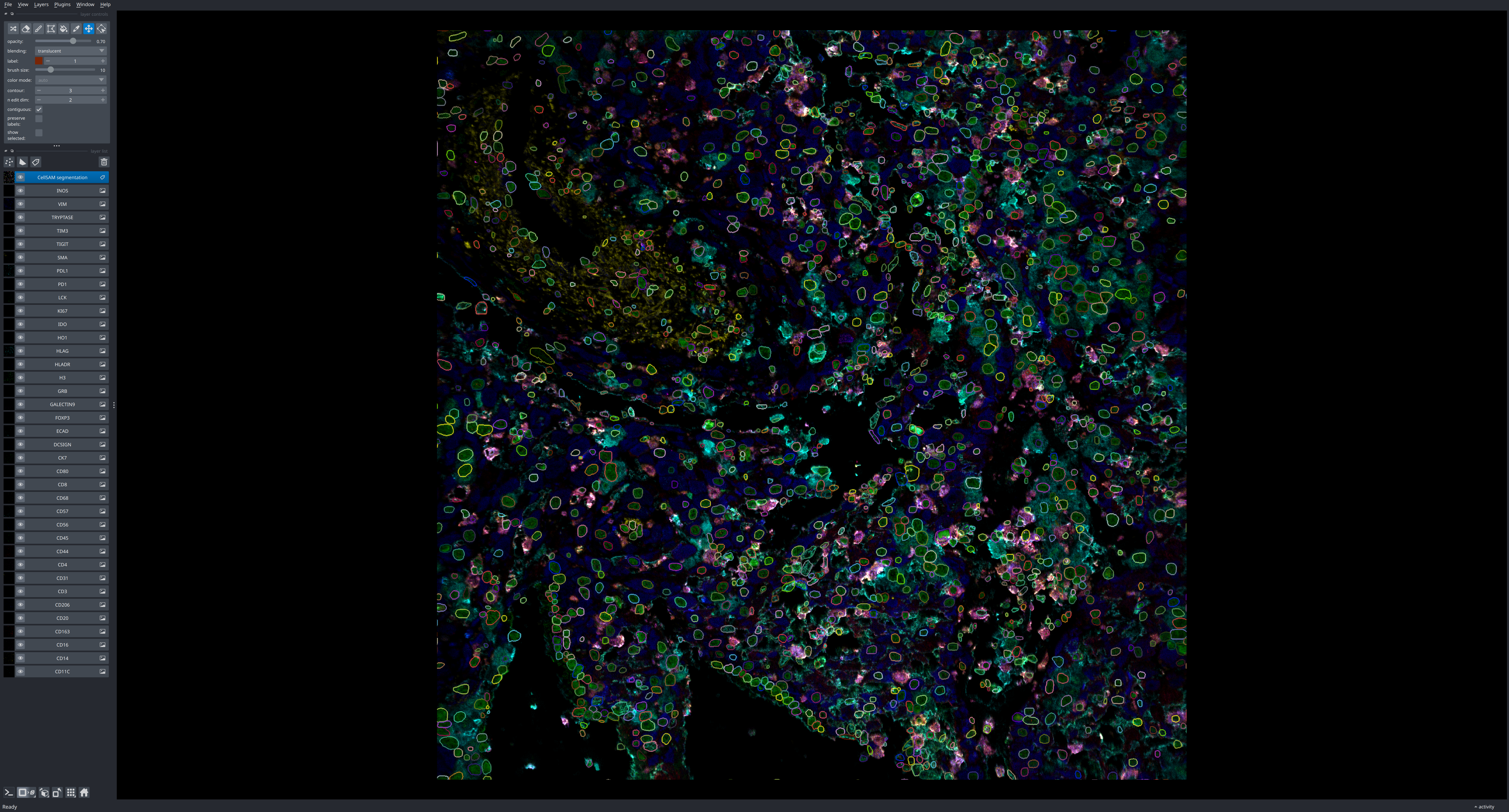
mask_lyr = nim.add_labels(mask, name="CellSAM segmentation")
mask_lyr.contour = 3  # Relatively thick borders for static viz

Show code cell content

Hide code cell content

# For static rendering - can safely be ignored if running notebook interactively
from pathlib import Path

screenshot_path = Path("../_static/_generated")
screenshot_path.mkdir(parents=True, exist_ok=True)
nim.screenshot(
    path=screenshot_path / "napari_img_and_segmentation.png",
    canvas_only=False,
);

Cell-type inference with deepcell-types

We now have all the necessary components to run the cell-type inference pipeline.

import deepcell_types

To run the inference pipeline, you will need a trained model. The download_model helper fetches the checkpoint to $HOME/.deepcell/models and returns the local path (it requires a DEEPCELL_ACCESS_TOKEN; see Models for details). The returned path can be passed straight to predict as model_name.

from deepcell_types.utils import download_model

# Downloads to $HOME/.deepcell/models on first call; subsequent calls reuse
# the cached checkpoint and return its path immediately.
model = download_model(version="2026-06-15")

# System-specific configuration

# Pick a device: the default GPU if one is available, otherwise the CPU
# (inference works the same on CPU, just slower). Use "cuda:1", "cuda:2",
# etc. to target a specific GPU.
import torch

device = "cuda" if torch.cuda.is_available() else "cpu"
# NOTE: For machines with many cores & large RAM (e.g. GPU nodes), consider
# increasing for better performance.
num_data_loader_threads = 1

The marker and cell-type registry the model needs is shipped with the package, so no additional data is required to run inference. If you instead want to source the registry from a local TissueNet zarr archive, pass zarr_path="/path/to/tissuenet.zarr" to predict (or set the DEEPCELL_TYPES_ZARR_PATH environment variable); the archive’s root attrs must define the same standardized marker and cell-type registry the checkpoint was trained against.

With the system all configured, we can now run the pipeline:

cell_types = deepcell_types.predict(
    img,
    mask,
    chnames,
    mpp,
    model_name=model,
    device=device,
    num_workers=num_data_loader_threads,
)

Show code cell output

Hide code cell output

Predictions are provided in the form of list of strings, where the order of the list is given by the ascending order of cell indices in the segmentation mask. Since we ordered the mask indices above, it’s straightforward to make this mapping explicit:

Note

Low-confidence abstention. Abstention is opt-in. By default (ct_abstention_k=0) predict returns the raw argmax label for every cell. To enable it, pass a positive float k: predict then flags cells whose top-class probability falls below an IQR fence on the field-of-view’s confidence distribution and rewrites their label to the sentinel "Unknown". Reported results use full coverage (no abstention). The following example shows how to opt into an IQR-fence threshold with k=0.2:

cell_types = deepcell_types.predict(
    img, mask, chnames, mpp,
    model_name=model, device=device,
    ct_abstention_k=0.2,
)

To inspect probabilities and which cells were abstained, pass return_probabilities=True to receive a PredictionResult with the full per-cell softmax matrix, the cell indices, a boolean abstained array, and the pre-abstention cell_types_raw labels.

idx_to_pred = dict(enumerate(cell_types, start=1))

pd.DataFrame.from_dict(  # For nice table rendering
    idx_to_pred, orient="index", columns=["Cell type"]
)

	Cell type
1	SmoothMuscle
2	Fibroblast
3	EVT
4	SmoothMuscle
5	EVT
...	...
1739	NK
1740	NK
1741	EVT
1742	NK
1743	Fibroblast

1743 rows × 1 columns

Depending on the subsequent analysis you wish to perform, it may be convenient to group the cells by their predicted cell-type:

from collections import defaultdict

# Convert the 1-1 `cell: type` mapping to a 1-many `type: list-of-cells` mapping
labels_by_celltype = defaultdict(list)
for idx, ct in idx_to_pred.items():
    labels_by_celltype[ct].append(idx)

Here’s the distribution of predicted cell types for this tissue:

from pprint import pprint

print(f"Total number of cells: {(num_cells := np.max(mask))}")

pprint(
    {
        k: f"{len(v)} ({100 * len(v) / num_cells:02.2f}%)"
        for k, v in labels_by_celltype.items()
    },
    sort_dicts=False,
)

Total number of cells: 1743
{'SmoothMuscle': '219 (12.56%)',
 'Fibroblast': '450 (25.82%)',
 'EVT': '295 (16.92%)',
 'Macrophage': '264 (15.15%)',
 'NK': '360 (20.65%)',
 'Epithelial': '92 (5.28%)',
 'Endothelial': '39 (2.24%)',
 'CD4T': '12 (0.69%)',
 'NKT': '2 (0.11%)',
 'CD8T': '9 (0.52%)',
 'Mast': '1 (0.06%)'}

Visualizing the results

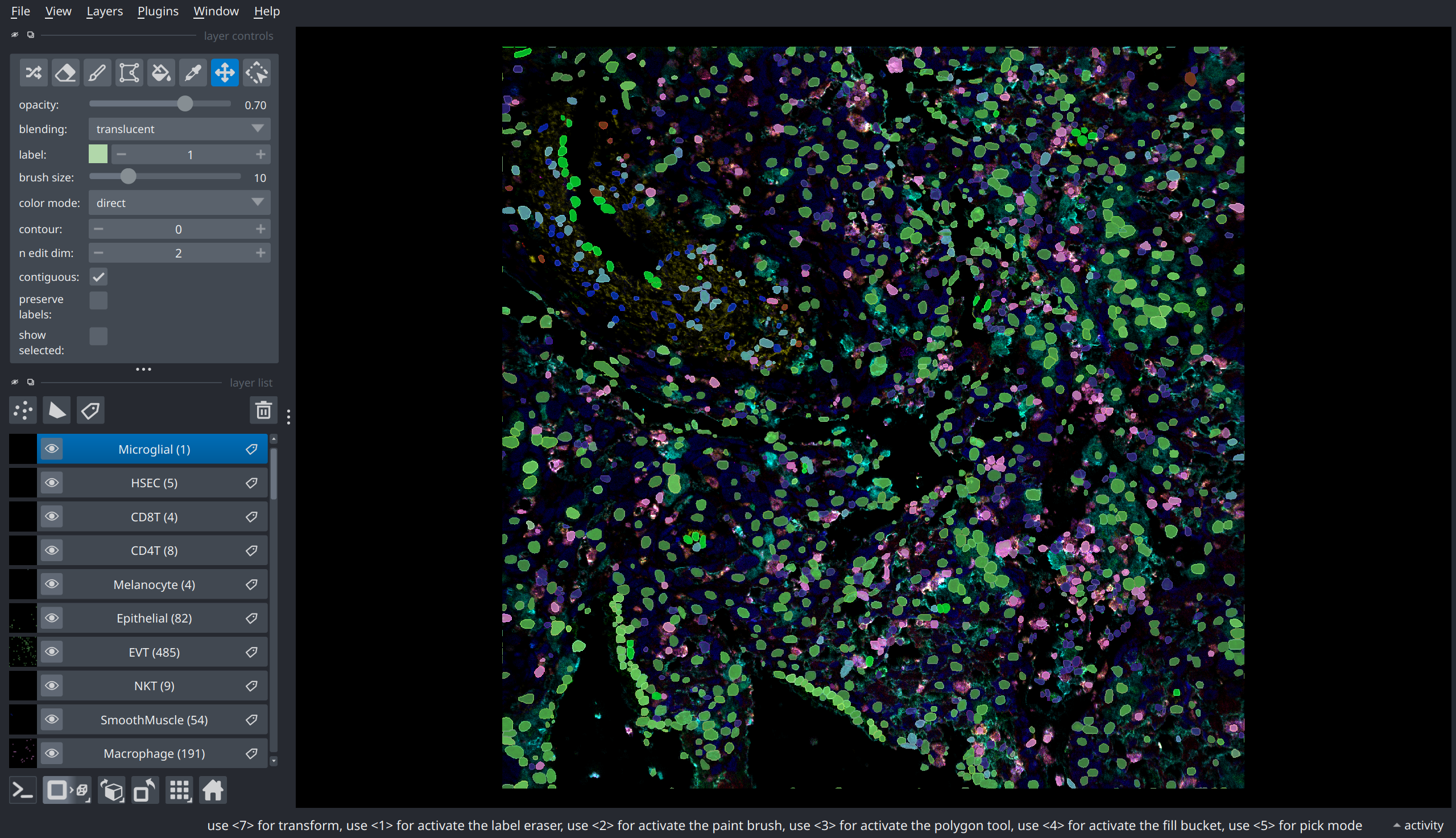
There are many ways to visualize the cell-type prediction data, each with their own advantages and disadvantages. One way is to add an independent layer for each predicted cell type. The advantage of this approach is that individual layers can be toggled to focus on a particular cell type during interactive visualization.

# Regionprops to extract slices corresponding to each individual cell mask
props = skimage.measure.regionprops(mask)
prop_dict = {p.label: p for p in props}

# Create a binary mask layer for each celltype and populate it
# using the regionprops
for k, l in labels_by_celltype.items():
    ctmask = np.zeros_like(mask, dtype=np.uint8)
    for idx in l:
        p = prop_dict[idx]
        ctmask[p.slice][p.image] = 1
    mask_lyr = nim.add_labels(ctmask, name=f"{k} ({len(l)})")
    mask_lyr.colormap = napari.utils.DirectLabelColormap(
        color_dict={None: (0, 0, 0), 1: np.random.rand(3)}
    )

Show code cell content

Hide code cell content

# For static rendering - can safely be ignored if running notebook interactively
from pathlib import Path

screenshot_path = Path("../_static/_generated")
screenshot_path.mkdir(parents=True, exist_ok=True)
nim.screenshot(
    path=screenshot_path / "napari_celltype_layers.png",
    canvas_only=False,
);