Data Science in Python#


Introduction#
Python is a general-purpose programming language and with the addition of a few popular libraries like numpy and scipy, has become a powerful scientific computing environment.
This notebook walks through some Python basics and an introduction to the computing libraries.
Those with previous coding experience in Matlab may find the NumPy for Matlab users page hepful.
In this tutorial, we will cover:
Basic Python: Data Structures (Containers, Lists, Dictionaries, Sets, Tuples), Functions, Classes
Basic Python: Control and Flow Statements
Installing Packages
Numpy: Arrays, Array Indexing, Datatypes, Array Math, Broadcasting
Matplotlib: Plotting, Subplots, Images
SciPy: Distance Between Points
Basics of Python#
Python is a high-level, dynamically-typed, object-oriented programming language. More to the point, Python code often appears very similar pseudocode and is more or less human-readable. As an example, here is an implementation of the classic quicksort algorithm in Python:
def quicksort(arr):
    if len(arr) <= 1:
        return arr
    pivot = arr[len(arr) // 2]
    left = [x for x in arr if x < pivot]
    middle = [x for x in arr if x == pivot]
    right = [x for x in arr if x > pivot]
    return quicksort(left) + middle + quicksort(right)

print(quicksort([3,6,8,10,1,2,1]))
[1, 1, 2, 3, 6, 8, 10]
Note: while most programming languages ignore whitespace and allow coders to put spaces, tabs, and newlines wherever they like in order to make their code readable, Python is different. In Python, indentation levels matter and each line of your code must be indented properly for it to run. Don’t worry, though. You’ll have an intuitive understanding of how to indent your Python code in no time.
Other note: there are two different supported versions of Python: 2.# and 3.#. The two version are not compatible with one another, so code written for 2.# may not work under 3.# and vice versa. DeepCell is written in python 3, so all code in this tutorial will use Python 3.7.
You can check your Python version at the command line by running python --version.
Section 1: Variable Types and Data Structures#
Numbers#
Integers and floats work as you would expect from other languages:
x = 3
print(x)
type(x)
3
int
print(x + 1)   # Addition;
print(x - 1)   # Subtraction;
print(x * 2)   # Multiplication;
print(x ** 2)  # Exponentiation;
4
2
6
9
x += 1
print(x)  # Prints "4"
x *= 2
print(x)  # Prints "8"
4
8
y = 2.5
print(type(y)) # Prints "<class 'float'>"
print(y, y + 1, y * 2, y ** 2)# Prints "2.5 3.5 5.0 6.25"
<class 'float'>
2.5 3.5 5.0 6.25
Note that unlike many languages, Python does not have unary increment (x++) or decrement (x–) operators.
Python also has built-in types for long integers and complex numbers; you can find all of the details in the documentation.
Booleans#
Python implements all of the usual operators for Boolean logic, but uses English words rather than symbols (&&, ||, etc.):
t, f = True, False
print(type(t)) # Prints "<type 'bool'>"
<class 'bool'>
Now we let’s look at the operations:
print(t and f) # Logical AND;
print(t or f)  # Logical OR;
print(not t)   # Logical NOT;
print(t != f)  # Logical XOR;
False
True
False
True
Strings#
hello = 'hello'   # String literals can use single quotes
world = "world"   # or double quotes; it does not matter.
print(hello, len(hello))
hello 5
hw = hello + ' ' + world  # String concatenation
print(hw)  # prints "hello world"
hello world
hw12 = '%s %s %d' % (hello, world, 12)  # sprintf style string formatting
print(hw12)  # prints "hello world 12"
hello world 12
String objects have a bunch of useful methods; for example:
s = "hello"
print(s.capitalize())  # Capitalize a string; prints "Hello"
print(s.upper())       # Convert a string to uppercase; prints "HELLO"
print(s.rjust(7))      # Right-justify a string, padding with spaces; prints "  hello"
print(s.center(7))     # Center a string, padding with spaces; prints " hello "
print(s.replace('l', '(ell)'))  # prints "he(ell)(ell)o"
print( '  world '.strip())  # Strip leading and trailing whitespace; prints "world"
Hello
HELLO
  hello
 hello
he(ell)(ell)o
world
You can find a list of all string methods in the documentation.
Containers#
Containers are objects which contain multiple other objects. Python includes several built-in container types: lists, dictionaries, sets, and tuples.
Lists#
A list is the Python equivalent of an array, but is resizeable and can contain elements of different types:
xs = [3, 1, 2]   # Create a list
print(xs, xs[2])
print(xs[-1])     # Negative indices count from the end of the list; prints "2"
[3, 1, 2] 2
2
xs[2] = 'foo'    # Lists can contain elements of different types
print(xs)
[3, 1, 'foo']
xs.append('bar') # Add a new element to the end of the list
print(xs)
[3, 1, 'foo', 'bar']
x = xs.pop()     # Remove and return the last element of the list
print(x, xs)
bar [3, 1, 'foo']
As always, more information is available in the documentation.
Slicing is an operation performed on lists.
In addition to accessing list elements one at a time, Python provides concise syntax to access sublists; this is known as slicing:
nums = list(range(5))
print(nums)          # Prints "[0, 1, 2, 3, 4]"
print(nums[2:4])     # Get a slice from index 2 to 4 (exclusive); prints "[2, 3]"
print(nums[2:])      # Get a slice from index 2 to the end; prints "[2, 3, 4]"
print(nums[:2])      # Get a slice from the start to index 2 (exclusive); prints "[0, 1]"
print(nums[:])       # Get a slice of the whole list; prints ["0, 1, 2, 3, 4]"
print(nums[:-1] )    # Slice indices can be negative; prints ["0, 1, 2, 3]"
nums[2:4] = [8, 9]   # Assign a new sublist to a slice
print(nums)          # Prints "[0, 1, 8, 9, 4]"
[0, 1, 2, 3, 4]
[2, 3]
[2, 3, 4]
[0, 1]
[0, 1, 2, 3, 4]
[0, 1, 2, 3]
[0, 1, 8, 9, 4]
Looping is an operation performed on lists, too. You can loop over the elements of a list like this:
animals = ['cat', 'dog', 'monkey']
for animal in animals:
    print(animal)
cat
dog
monkey
If you want access to the index of each element within the body of a loop, use the built-in enumerate function:
animals = ['cat', 'dog', 'monkey']
for idx, animal in enumerate(animals):
    print('#%d: %s' % (idx + 1, animal))
#1: cat
#2: dog
#3: monkey
A cool way of modifying a list is by using a “list comprehension”.
When programming, frequently we want to transform one type of data into another. As a simple example, consider the following code that computes the square of numbers in a list:
nums = [0, 1, 2, 3, 4]
squares = []
for x in nums:
    squares.append(x ** 2)
print(squares)
[0, 1, 4, 9, 16]
You can make this code simpler using a list comprehension:
nums = [0, 1, 2, 3, 4]
squares = [x ** 2 for x in nums]
print(squares)
[0, 1, 4, 9, 16]
List comprehensions can also contain conditions:
nums = [0, 1, 2, 3, 4]
even_squares = [x ** 2 for x in nums if x % 2 == 0]
print(even_squares)
[0, 4, 16]
Dictionaries#
A dictionary stores (key, value) pairs, similar to an object in Javascript. You can use it like this:
d = {'cat': 'sad', 'dog': 'furry'}  # Create a new dictionary with some data
print(d['cat'])       # Get an entry from a dictionary; prints "cute"
print('cat' in d)     # Check if a dictionary has a given key; prints "True"
sad
True
d['fish'] = 'wet'    # Set an entry in a dictionary
print(d['fish'])      # Prints "wet"
wet
print(d['monkey']) # KeyError: 'monkey' not a key of d
---------------------------------------------------------------------------
KeyError                                  Traceback (most recent call last)
<ipython-input-24-78fc9745d9cf> in <module>()
----> 1 print(d['monkey'])  # KeyError: 'monkey' not a key of d

KeyError: 'monkey'
print(d.get('monkey', 'N/A'))  # Get an element with a default; prints "N/A"
print(d.get('fish', 'N/A'))    # Get an element with a default; prints "wet"
N/A
wet
del d['fish']        # Remove an element from a dictionary
print(d.get('fish', 'N/A')) # "fish" is no longer a key; prints "N/A"
It is easy to iterate over the keys in a dictionary:
d = {'person': 2, 'cat': 4, 'spider': 8}
for animal in d:
    legs = d[animal]
    print('A %s has %d legs' % (animal, legs))
A person has 2 legs
A cat has 4 legs
A spider has 8 legs
If you want access to keys and their corresponding values, use the items method:
d = {'person': 2, 'cat': 4, 'spider': 8}
for animal, legs in d.items():
    print('A %s has %d legs' % (animal, legs))
A person has 2 legs
A cat has 4 legs
A spider has 8 legs
Dictionary comprehensions: These are similar to list comprehensions, but allow you to easily construct dictionaries. For example:
nums = [0, 1, 2, 3, 4]
even_num_to_square = {x: x ** 2 for x in nums if x % 2 == 0}
print(even_num_to_square)
{0: 0, 2: 4, 4: 16}
More information on dictionaries is available in the documentation.
Sets#
A set is an unordered collection of distinct elements. As a simple example, consider the following:
animals = {'cat', 'dog'}
print('cat' in animals)   # Check if an element is in a set; prints "True"
print('fish' in animals)  # prints "False"
True
False
animals.add('fish')      # Add an element to a set
print('fish' in animals)
print(len(animals))       # Number of elements in a set;
True
3
animals.add('cat')       # Adding an element that is already in the set does nothing
print(len(animals))
animals.remove('cat')    # Remove an element from a set
print(len(animals))
3
2
Loops: Iterating over a set has the same syntax as iterating over a list; however since sets are unordered, you cannot make assumptions about the order in which you visit the elements of the set:
animals = {'cat', 'dog', 'fish'}
for idx, animal in enumerate(animals):
    print('#%d: %s' % (idx + 1, animal))
# Prints "#1: fish", "#2: dog", "#3: cat"
#1: fish
#2: cat
#3: dog
Set comprehensions: Like lists and dictionaries, we can easily construct sets using set comprehensions:
from math import sqrt
print({int(sqrt(x)) for x in range(30)})
{0, 1, 2, 3, 4, 5}
Tuples#
A tuple is an (immutable) ordered list of values. A tuple is in many ways similar to a list; one of the most important differences is that tuples can be used as keys in dictionaries and as elements of sets, while lists cannot. Here is a trivial example:
d = {(x, x + 1): x for x in range(10)}  # Create a dictionary with tuple keys
print(d)
t = (5, 6)       # Create a tuple
print(type(t))
print(d[t])
print(d[(1, 2)])
{(0, 1): 0, (1, 2): 1, (2, 3): 2, (3, 4): 3, (4, 5): 4, (5, 6): 5, (6, 7): 6, (7, 8): 7, (8, 9): 8, (9, 10): 9}
<class 'tuple'>
5
1
t[0] = 1
---------------------------------------------------------------------------
TypeError                                 Traceback (most recent call last)
<ipython-input-35-c8aeb8cd20ae> in <module>()
----> 1 t[0] = 1

TypeError: 'tuple' object does not support item assignment
Functions#
Python functions are defined using the def keyword. For example:
def sign(x):
    if x > 0:
        return 'positive'
    elif x < 0:
        return 'negative'
    else:
        return 'zero'

for x in [-1, 0, 1]:
    print(sign(x))
negative
zero
positive
We will often define functions to take optional keyword arguments, like this:
def hello(name, loud=False):
    if loud:
        print('HELLO, %s' % name.upper())
    else:
        print('Hello, %s!' % name)

hello('Bob')
hello('Fred', loud=True)
Hello, Bob!
HELLO, FRED
Classes#
The syntax for defining classes in Python is straightforward:
class Greeter:

    # Constructor (Really more of Initializer as object already exists)
    def __init__(self, name):
        self.name = name  # Create an instance variable

    # Instance method
    def greet(self, loud=False):
        if loud:
            print('HELLO, %s!' % self.name.upper())
        else:
            print('Hello, %s' % self.name)

g = Greeter('Fred')  # Construct an instance of the Greeter class
g.greet()            # Call an instance method; prints "Hello, Fred"
g.greet(loud=True)   # Call an instance method; prints "HELLO, FRED!"
Hello, Fred
HELLO, FRED!
Section 2: Control and Flow Statements#
We’ve seen a few if and for statements already, but let’s explicitly describe them before we move on to the various libraries (or Python “add-ons” if you will) we will be using.
The key thing to note about Python’s control flow statements and program structure is that it uses indentations to mark blocks. So the number of spaces at the start of a line is very important.
Conditionals: if and else#
if some_condition:
    code block
x = 12
if x > 10:
    print("Hello")
Hello
if-else:
if some_condition:
    algorithm
else:
    algorithm
x = 12
if 10 < x < 11:
    print("hello")
else:
    print("world")
world
OR: else-if
if some_condition:
    algorithm
elif some_condition:
    algorithm
else:
    algorithm
x = 10
y = 12
if x > y:
    print("x>y")
elif x < y:
    print("x<y")
else:
    print("x=y")
x<y
Loops#
for variable in something:
    algorithm
As we’ve already seen, when looping over integers the range() function is useful which generates a range of integers:
range(n) = 0, 1, …, n-1
range(m,n)= m, m+1, …, n-1
range(m,n,s)= m, m+s, m+2s, …, m + ((n-m-1)//s) * s
for ch in 'abc':
    print(ch)
total = 0
for i in range(5):
    total += i
for i,j in [(1,2),(3,1)]:
    total += i**j
print("total =",total)
a
b
c
total = 14
while some_condition:
    algorithm
i = 1
while i < 3:
    print(i ** 2)
    i = i+1
print('Bye')
1
4
Bye
Breaks and Continues#
As the name implies, a break statement is used to break out of a loop when a condition becomes true when executing the loop.
for i in range(100):
    print(i)
    if i>=7:
        break
0
1
2
3
4
5
6
7
This continues the rest of the loop. Sometimes when a condition is satisfied there are chances of the loop getting terminated. This can be avoided using continue statement.
for i in range(10):
    if i>4:
        print("Ignored",i)
        continue
    # this statement is not reach if i > 4
    print("Processed",i)
Processed 0
Processed 1
Processed 2
Processed 3
Processed 4
Ignored 5
Ignored 6
Ignored 7
Ignored 8
Ignored 9
Catching Exceptions#
To break out of deeply nested execution sometimes it is useful to raise an exception. A try block allows you to catch exceptions that happen anywhere during the execution of the try block:
try:
    code
except <Exception Type> as <variable name>:
    # deal with error of this type
except:
    # deal with any error
These statements can be a graceful way of dealing with system errors
try:
    count=0
    while True:
        while True:
            while True:
                print("Looping")
                count = count + 1
                if count > 3:
                    raise Exception("abort") # exit every loop or function
except Exception as e: # this is where we go when an exception is raised
    print("Caught exception:",e)
Looping
Looping
Looping
Looping
Caught exception: abort
Section 3: Installing Packages#
Out of the box, Python comes with a lot of cool functionality for manipulating text files, interfacing with the operating system, keeping track of time…
Ok, so not a lot of flashy stuff. BUT there are tons of packages that can do very cool things!
We will look at three of them in the following sections. However, to use a Python package, you first have to install it.
If you installed Python on the command line, then execute the following commands:
pip install numpy
pip install matplotlib
pip install scipy
If you installed Anaconda Python, then execute these commands:
conda install numpy
conda install matplotlib
conda install scipy
Section 4: NumPy#
NumPy is the core library for scientific computing in Python. It provides a high-performance multidimensional array object and tools for working with these arrays. If you are already familiar with MATLAB, you might find this tutorial useful to get started with Numpy.
To use NumPy, we first need to import the numpy package:
import numpy as np
Arrays#
A numpy array is a grid of values, all of the same type, and is indexed by a tuple of nonnegative integers. The number of dimensions is the rank of the array; the shape of an array is a tuple of integers giving the size of the array along each dimension.
We can initialize numpy arrays from nested Python lists, and access elements using square brackets:
a = np.array([1, 2, 3])  # Create a rank 1 array
print(type(a), a.shape, a[0], a[1], a[2])
a[0] = 5                 # Change an element of the array
print(a)
<class 'numpy.ndarray'> (3,) 1 2 3
[5 2 3]
b = np.array([[1,2,3],[4,5,6]])   # Create a rank 2 array
print(b)
[[1 2 3]
 [4 5 6]]
print(b.shape)
print(b[0, 0], b[0, 1], b[1, 0])
(2, 3)
1 2 4
Numpy also provides many functions to create arrays:
a = np.zeros((2,2))  # Create an array of all zeros
print(a)
[[0. 0.]
 [0. 0.]]
b = np.ones((1,2))   # Create an array of all ones
print(b)
[[1. 1.]]
c = np.full((2,2), 7) # Create a constant array
print(c)
[[7 7]
 [7 7]]
d = np.eye(2)        # Create a 2x2 identity matrix
print(d)
[[1. 0.]
 [0. 1.]]
e = np.random.random((2,2)) # Create an array filled with random values
print(e)
[[0.48053284 0.91259894]
 [0.40260486 0.31897294]]
N.B. numpy.random.random is an alias for numpy.random.random_sample.
Array indexing#
Numpy offers several ways to index into arrays.
Slicing: Similar to Python lists, numpy arrays can be sliced. Since arrays may be multidimensional, you must specify a slice for each dimension of the array:
import numpy as np

# Create the following rank 2 (2-dimensional) array with shape (3, 4)
# [[ 1  2  3  4]
#  [ 5  6  7  8]
#  [ 9 10 11 12]]
a = np.array([[1,2,3,4], [5,6,7,8], [9,10,11,12]])

# Use slicing to pull out the subarray consisting of the first 2 rows
# and columns 1 and 2; b is the following array of shape (2, 2):
# [[2 3]
#  [6 7]]
b = a[:2, 1:3]
print(b)
print(b.shape)
[[2 3]
 [6 7]]
(2, 2)
A slice of an array is a view into the same data, so modifying it will modify the original array.
print(a[0, 1])
b[0, 0] = 77    # b[0, 0] is the same piece of data as a[0, 1]
print(a[0, 1])
2
77
You can also mix integer indexing with slice indexing. However, doing so will yield an array of lower rank than the original array. Note that this is quite different from the way that MATLAB handles array slicing:
# Create the following rank 2 array with shape (3, 4)
a = np.array([[1,2,3,4], [5,6,7,8], [9,10,11,12]])
print(a)
[[ 1  2  3  4]
 [ 5  6  7  8]
 [ 9 10 11 12]]
Two ways of accessing the data in the middle row of the array. Mixing integer indexing with slices yields an array of lower rank, while using only slices yields an array of the same rank as the original array:
row_r1 = a[1, :]    # Rank 1 view of the second row of a
row_r2 = a[1:2, :]  # Rank 2 view of the second row of a
row_r3 = a[[1], :]  # Rank 2 view of the second row of a
print(row_r1, row_r1.shape)
print(row_r2, row_r2.shape)
print(row_r3, row_r3.shape)
[5 6 7 8] (4,)
[[5 6 7 8]] (1, 4)
[[5 6 7 8]] (1, 4)
# We can make the same distinction when accessing columns of an array:
col_r1 = a[:, 1]
col_r2 = a[:, 1:2]
print(col_r1, col_r1.shape)
print(col_r2, col_r2.shape)
[ 2  6 10] (3,)
[[ 2]
 [ 6]
 [10]] (3, 1)
Integer array indexing: When you index into numpy arrays using slicing, the resulting array view will always be a subarray of the original array. In contrast, integer array indexing allows you to construct arbitrary arrays using the data from another array. Here is an example:
a = np.array([[1, 2], [3, 4], [5, 6]])

# An example of integer array indexing.
# The returned array will have shape (3,) and
print(a[[0, 1, 2], [0, 1, 0]])

# The above example of integer array indexing is equivalent to this:
print(np.array([a[0, 0], a[1, 1], a[2, 0]]))
[1 4 5]
[1 4 5]
# When using integer array indexing, you can reuse the same
# element from the source array:
print(a[[0, 0], [1, 1]])

# Equivalent to the previous integer array indexing example
print(np.array([a[0, 1], a[0, 1]]))
[2 2]
[2 2]
One useful trick with integer array indexing is selecting or mutating one element from each row of a matrix:
# Create a new array from which we will select elements
a = np.array([[1,2,3], [4,5,6], [7,8,9], [10, 11, 12]])
print(a)
[[ 1  2  3]
 [ 4  5  6]
 [ 7  8  9]
 [10 11 12]]
# Create an array of indices
b = np.array([0, 2, 0, 1])

# Select one element from each row of a using the indices in b
print(a[np.arange(4), b])  # Prints "[ 1  6  7 11]"
[ 1 6 7 11]
# Mutate one element from each row of a using the indices in b
a[np.arange(4), b] += 10
print(a)
[[11  2  3]
 [ 4  5 16]
 [17  8  9]
 [10 21 12]]
Boolean array indexing: Boolean array indexing lets you pick out arbitrary elements of an array. Frequently this type of indexing is used to select the elements of an array that satisfy some condition. Here is an example:
import numpy as np

a = np.array([[1,2], [3, 4], [5, 6]])

bool_idx = (a > 2)  # Find the elements of a that are bigger than 2;
                    # this returns a numpy array of Booleans of the same
                    # shape as a, where each slot of bool_idx tells
                    # whether that element of a is > 2.

print(bool_idx)
[[False False]
 [ True  True]
 [ True  True]]
# We use boolean array indexing to construct a rank 1 array
# consisting of the elements of a corresponding to the True values
# of bool_idx
print(a[bool_idx])

# We can do all of the above in a single concise statement:
print(a[a > 2])
[3 4 5 6]
[3 4 5 6]
For brevity we have left out a lot of details about numpy array indexing; if you want to know more you should read the documentation.
Datatypes#
Every numpy array is a grid of elements of the same type. Numpy provides a large set of numeric datatypes that you can use to construct arrays. Numpy tries to guess a datatype when you create an array, but functions that construct arrays usually also include an optional argument to explicitly specify the datatype. Here is an example:
x = np.array([1, 2])  # Let numpy choose the datatype
y = np.array([1.0, 2.0])  # Let numpy choose the datatype
z = np.array([1, 2], dtype=np.int64)  # Force a particular datatype

print(x.dtype, y.dtype, z.dtype)
int64 float64 int64
You can read all about numpy datatypes in the documentation.
Array math#
Basic mathematical functions operate elementwise on arrays, and are available both as operator overloads and as functions in the numpy module:
x = np.array([[1,2],[3,4]], dtype=np.float64)
y = np.array([[5,6],[7,8]], dtype=np.float64)

# Elementwise sum; both produce the array
print(x + y)
print(np.add(x, y))
[[ 6.  8.]
 [10. 12.]]
[[ 6.  8.]
 [10. 12.]]
# Elementwise difference; both produce the array
print(x - y)
print(np.subtract(x, y))
[[-4. -4.]
 [-4. -4.]]
[[-4. -4.]
 [-4. -4.]]
# Elementwise product; both produce the array
print(x * y)
print(np.multiply(x, y))
[[ 5. 12.]
 [21. 32.]]
[[ 5. 12.]
 [21. 32.]]
# Elementwise division; both produce the array
# [[ 0.2         0.33333333]
#  [ 0.42857143  0.5       ]]
print(x / y)
print(np.divide(x, y))
[[0.2        0.33333333]
 [0.42857143 0.5       ]]
[[0.2        0.33333333]
 [0.42857143 0.5       ]]
# Elementwise square root; produces the array
# [[ 1.          1.41421356]
#  [ 1.73205081  2.        ]]
print(np.sqrt(x))
[[1.         1.41421356]
 [1.73205081 2.        ]]
Note that unlike MATLAB, * is elementwise multiplication, not matrix multiplication. We instead use the dot function to compute inner products of vectors, to multiply a vector by a matrix, and to multiply matrices. dot is available both as a function in the numpy module and as an instance method of array objects:
x = np.array([[1,2],[3,4]])
y = np.array([[5,6],[7,8]])

v = np.array([9,10])
w = np.array([11, 12])

# Inner product of vectors; both produce 219
print(v.dot(w))
print(np.dot(v, w))
219
219
# Matrix / vector product; both produce the rank 1 array [29 67]
print(x.dot(v))
print(np.dot(x, v))
[29 67]
[29 67]
# Matrix / matrix product; both produce the rank 2 array
# [[19 22]
#  [43 50]]
print(x.dot(y))
print(np.dot(x, y))
[[19 22]
 [43 50]]
[[19 22]
 [43 50]]
Numpy provides many useful functions for performing computations on arrays; one of the most useful is sum:
x = np.array([[1,2],[3,4]])

print(np.sum(x))  # Compute sum of all elements; prints "10"
print(np.sum(x, axis=0))  # Compute sum of each column; prints "[4 6]"
print(np.sum(x, axis=1))  # Compute sum of each row; prints "[3 7]"
10
[4 6]
[3 7]
You can find the full list of mathematical functions provided by numpy in the documentation.
Apart from computing mathematical functions using arrays, we frequently need to reshape or otherwise manipulate data in arrays. The simplest example of this type of operation is transposing a matrix; to transpose a matrix, simply use the T attribute of an array object:
print(x)
print(x.T)
[[1 2]
 [3 4]]
[[1 3]
 [2 4]]
v = np.array([[1,2,3]])
print(v)
print(v.T)
[[1 2 3]]
[[1]
 [2]
 [3]]
Broadcasting#
Broadcasting is a powerful mechanism that allows numpy to work with arrays of different shapes when performing arithmetic operations. Frequently, we have a smaller array and a larger array, and we want to use the smaller array multiple times to perform some operation on the larger array.
For example, suppose that we want to add a constant vector to each row of a matrix. We could do it like this:
# We will add the vector v to each row of the matrix x,
# storing the result in the matrix y
x = np.array([[1,2,3], [4,5,6], [7,8,9], [10, 11, 12]])
print(x)
v = np.array([1, 0, 1])
print(v)
y = np.empty_like(x)   # Create an empty matrix with the same shape as x

# Add the vector v to each row of the matrix x with an explicit loop
for i in range(4):
    y[i, :] = x[i, :] + v

print(y)
[[ 1  2  3]
 [ 4  5  6]
 [ 7  8  9]
 [10 11 12]]
[1 0 1]
[[ 2  2  4]
 [ 5  5  7]
 [ 8  8 10]
 [11 11 13]]
While this works, when the matrix x is very large, computing an explicit loop in Python could be slow. Note that adding the vector v to each row of the matrix x is equivalent to forming a matrix vv by stacking multiple copies of v vertically, then performing elementwise summation of x and vv. We could implement this approach like this:
vv = np.tile(v, (4, 1))  # Stack 4 copies of v on top of each other
print(vv)                 # Prints "[[1 0 1]
                         #          [1 0 1]
                         #          [1 0 1]
                         #          [1 0 1]]"
[[1 0 1]
 [1 0 1]
 [1 0 1]
 [1 0 1]]
y = x + vv  # Add x and vv elementwise
print(y)
[[ 2  2  4]
 [ 5  5  7]
 [ 8  8 10]
 [11 11 13]]
Numpy broadcasting allows us to perform this computation without actually creating multiple copies of v. Consider this version, using broadcasting:
import numpy as np

# We will add the vector v to each row of the matrix x,
# storing the result in the matrix y
x = np.array([[1,2,3], [4,5,6], [7,8,9], [10, 11, 12]])
v = np.array([1, 0, 1])
y = x + v  # Add v to each row of x using broadcasting
print(y)
[[ 2  2  4]
 [ 5  5  7]
 [ 8  8 10]
 [11 11 13]]
The line y = x + v works even though x has shape (4, 3) and v has shape (3,) due to broadcasting; this line works as if v actually had shape (4, 3), where each row was a copy of v, and the sum was performed elementwise.
Broadcasting two arrays together follows these rules:
If the arrays do not have the same rank, prepend the shape of the lower rank array with 1s until both shapes have the same length.
The two arrays are said to be compatible in a dimension if they have the same size in the dimension, or if one of the arrays has size 1 in that dimension.
The arrays can be broadcast together if they are compatible in all dimensions.
After broadcasting, each array behaves as if it had shape equal to the elementwise maximum of shapes of the two input arrays.
In any dimension where one array had size 1 and the other array had size greater than 1, the first array behaves as if it were copied along that dimension
If this explanation does not make sense, try reading the explanation from the documentation or this explanation.
Functions that support broadcasting are known as universal functions. You can find the list of all universal functions in the documentation.
Here are some applications of broadcasting:
# Compute outer product of vectors
v = np.array([1,2,3])  # v has shape (3,)
w = np.array([4,5])    # w has shape (2,)
# To compute an outer product, we first reshape v to be a column
# vector of shape (3, 1); we can then broadcast it against w to yield
# an output of shape (3, 2), which is the outer product of v and w:

print(np.reshape(v, (3, 1)) * w)
[[ 4  5]
 [ 8 10]
 [12 15]]
# Add a vector to each row of a matrix
x = np.array([[1,2,3], [4,5,6]])
# x has shape (2, 3) and v has shape (3,) so they broadcast to (2, 3),
# giving the following matrix:

print(x + v)
[[2 4 6]
 [5 7 9]]
# Add a vector to each column of a matrix
# x has shape (2, 3) and w has shape (2,).
# If we transpose x then it has shape (3, 2) and can be broadcast
# against w to yield a result of shape (3, 2); transposing this result
# yields the final result of shape (2, 3) which is the matrix x with
# the vector w added to each column. Gives the following matrix:

print((x.T + w).T)
[[ 5  6  7]
 [ 9 10 11]]
# Another solution is to reshape w to be a row vector of shape (2, 1);
# we can then broadcast it directly against x to produce the same
# output.
print(x + np.reshape(w, (2, 1)))
[[ 5  6  7]
 [ 9 10 11]]
# Multiply a matrix by a constant:
# x has shape (2, 3). Numpy treats scalars as arrays of shape ();
# these can be broadcast together to shape (2, 3), producing the
# following array:
print(x * 2)
[[ 2  4  6]
 [ 8 10 12]]
Broadcasting typically makes your code more concise and faster, so you should strive to use it where possible.
This brief overview has touched on many of the important things that you need to know about numpy, but is far from complete. Check out the numpy reference to find out much more about numpy.
Section 5: Matplotlib#
Matplotlib is a plotting library. In this section, we give a brief introduction to the matplotlib.pyplot module, which provides a plotting system similar to that of MATLAB.
import matplotlib.pyplot as plt
By running this special iPython command, we will be displaying plots inline:
%matplotlib inline
Plotting#
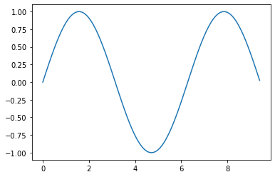
The most important function in matplotlib is plot, which allows you to plot 2D data. Here is a simple example:
# Compute the x and y coordinates for points on a sine curve
x = np.arange(0, 3 * np.pi, 0.1)
y = np.sin(x)

# Plot the points using matplotlib
plt.plot(x, y)
[<matplotlib.lines.Line2D at 0x7f2f2cb5b310>]
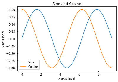
With just a little bit of extra work we can easily plot multiple lines at once, and add a title, legend, and axis labels:
y_sin = np.sin(x)
y_cos = np.cos(x)

# Plot the points using matplotlib
plt.plot(x, y_sin)
plt.plot(x, y_cos)
plt.xlabel('x axis label')
plt.ylabel('y axis label')
plt.title('Sine and Cosine')
plt.legend(['Sine', 'Cosine'])
<matplotlib.legend.Legend at 0x7f2f2cb797d0>
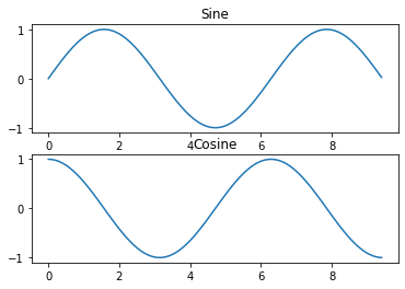
Subplots#
You can plot different things in the same figure using the subplot function. Here is an example:
# Compute the x and y coordinates for points on sine and cosine curves
x = np.arange(0, 3 * np.pi, 0.1)
y_sin = np.sin(x)
y_cos = np.cos(x)

# Set up a subplot grid that has height 2 and width 1,
# and set the first such subplot as active.
plt.subplot(2, 1, 1)

# Make the first plot
plt.plot(x, y_sin)
plt.title('Sine')

# Set the second subplot as active, and make the second plot.
plt.subplot(2, 1, 2)
plt.plot(x, y_cos)
plt.title('Cosine')

# Show the figure.
plt.show()
Alternatively the plt.subplots function creates a figure and an array of subplots which can be easily iterated over.
# Initialize a subplot grid with height 2 and width 1
fig,ax = plt.subplots(2,1)

# ax is an array object containing each subplot according to standard array indexing
ax[0].plot(x, y_sin)
ax[0].set_title('Sine')

ax[1].plot(x, y_cos)
ax[1].set_title('Cosine')
Text(0.5, 1.0, 'Cosine')
As always, you can read much more about the subplot function in the documentation. So far this is just a taste of what matplotlib can do for data visualization. Check out the gallery provided in matplotlib’s documentation for more examples.
Section 6: SciPy#
Numpy provides a high-performance multidimensional array and basic tools to compute with and manipulate these arrays. SciPy builds on this, and provides a large number of functions that operate on numpy arrays and are useful for different types of scientific and engineering applications.
Distance between points#
SciPy defines some useful functions for computing distances between sets of points.
The function scipy.spatial.distance.pdist computes the distance between all pairs of points in a given set:
import numpy as np
from scipy.spatial.distance import pdist, squareform

# Create the following array where each row is a point in 2D space:
# [[0 1]
#  [1 0]
#  [2 0]]
x = np.array([[0, 1], [1, 0], [2, 0]])
print(x)

# Compute the Euclidean distance between all rows of x.
# d[i, j] is the Euclidean distance between x[i, :] and x[j, :],
# and d is the following array:
# [[ 0.          1.41421356  2.23606798]
#  [ 1.41421356  0.          1.        ]
#  [ 2.23606798  1.          0.        ]]
d = squareform(pdist(x, 'euclidean'))
print(d)
[[0 1]
 [1 0]
 [2 0]]
[[0.         1.41421356 2.23606798]
 [1.41421356 0.         1.        ]
 [2.23606798 1.         0.        ]]
You can read all the details about this function in the documentation.
A similar function (scipy.spatial.distance.cdist) computes the distance between all pairs across two sets of points; you can read about it in the documentation.
The best way to get familiar with SciPy is to browse the documentation. Day 2 will highlight more parts of SciPy that you might find useful in developing for DeepCell.
Section 7: Pandas#
import pandas as pd
Pandas is a flexible and powerful tool for handling datasets in python. To explore its basic functionality, we’ll look at how it can be applied to a simple dataset about heart health borrowed from An Introduction to Statistical Learning, with applications in R (Springer, 2013) with permission from the authors: G. James, D. Witten, T. Hastie and R. Tibshirani. This csv is hosted online and we can use pandas read_csv function to directly retrieve the dataset.
df = pd.read_csv('https://www.statlearning.com/s/Heart.csv',index_col=0)
df
| Age | Sex | ChestPain | RestBP | Chol | Fbs | RestECG | MaxHR | ExAng | Oldpeak | Slope | Ca | Thal | AHD | |
|---|---|---|---|---|---|---|---|---|---|---|---|---|---|---|
| 1 | 63 | 1 | typical | 145 | 233 | 1 | 2 | 150 | 0 | 2.3 | 3 | 0.0 | fixed | No |
| 2 | 67 | 1 | asymptomatic | 160 | 286 | 0 | 2 | 108 | 1 | 1.5 | 2 | 3.0 | normal | Yes |
| 3 | 67 | 1 | asymptomatic | 120 | 229 | 0 | 2 | 129 | 1 | 2.6 | 2 | 2.0 | reversable | Yes |
| 4 | 37 | 1 | nonanginal | 130 | 250 | 0 | 0 | 187 | 0 | 3.5 | 3 | 0.0 | normal | No |
| 5 | 41 | 0 | nontypical | 130 | 204 | 0 | 2 | 172 | 0 | 1.4 | 1 | 0.0 | normal | No |
| ... | ... | ... | ... | ... | ... | ... | ... | ... | ... | ... | ... | ... | ... | ... |
| 299 | 45 | 1 | typical | 110 | 264 | 0 | 0 | 132 | 0 | 1.2 | 2 | 0.0 | reversable | Yes |
| 300 | 68 | 1 | asymptomatic | 144 | 193 | 1 | 0 | 141 | 0 | 3.4 | 2 | 2.0 | reversable | Yes |
| 301 | 57 | 1 | asymptomatic | 130 | 131 | 0 | 0 | 115 | 1 | 1.2 | 2 | 1.0 | reversable | Yes |
| 302 | 57 | 0 | nontypical | 130 | 236 | 0 | 2 | 174 | 0 | 0.0 | 2 | 1.0 | normal | Yes |
| 303 | 38 | 1 | nonanginal | 138 | 175 | 0 | 0 | 173 | 0 | 0.0 | 1 | NaN | normal | No |
303 rows × 14 columns
Pandas has two fundamental data structures: DataFrames and Series. DataFrames are often abbreviated as df and are made up of multiple Series. If we index into df to retrieve a single column, it is returned as a Series.
age = df['Age']
print(age)
print('\n',type(age))
1      63
2      67
3      67
4      37
5      41
       ..
299    45
300    68
301    57
302    57
303    38
Name: Age, Length: 303, dtype: int64

 <class 'pandas.core.series.Series'>
Boolean indexing can also be applied to dataframes to select restricted subsets of the dataframe. In this case, we will use df.loc to perform the indexing and select all cases where Age = 45.
df.loc[df['Age'] == 45]
| Age | Sex | ChestPain | RestBP | Chol | Fbs | RestECG | MaxHR | ExAng | Oldpeak | Slope | Ca | Thal | AHD | |
|---|---|---|---|---|---|---|---|---|---|---|---|---|---|---|
| 81 | 45 | 1 | asymptomatic | 104 | 208 | 0 | 2 | 148 | 1 | 3.0 | 2 | 0.0 | normal | No |
| 101 | 45 | 1 | asymptomatic | 115 | 260 | 0 | 2 | 185 | 0 | 0.0 | 1 | 0.0 | normal | No |
| 126 | 45 | 0 | nontypical | 130 | 234 | 0 | 2 | 175 | 0 | 0.6 | 2 | 0.0 | normal | No |
| 149 | 45 | 1 | nontypical | 128 | 308 | 0 | 2 | 170 | 0 | 0.0 | 1 | 0.0 | normal | No |
| 170 | 45 | 0 | nontypical | 112 | 160 | 0 | 0 | 138 | 0 | 0.0 | 2 | 0.0 | normal | No |
| 198 | 45 | 0 | asymptomatic | 138 | 236 | 0 | 2 | 152 | 1 | 0.2 | 2 | 0.0 | normal | No |
| 206 | 45 | 1 | asymptomatic | 142 | 309 | 0 | 2 | 147 | 1 | 0.0 | 2 | 3.0 | reversable | Yes |
| 299 | 45 | 1 | typical | 110 | 264 | 0 | 0 | 132 | 0 | 1.2 | 2 | 0.0 | reversable | Yes |
Pandas documentation covers a variety of other applications of boolean indexing and dataframes.
Inspecting Dataframes#
Pandas supplies several useful methods for quickly inspecting data:
# Calling the dataframe alone will show the first and last five rows
df
| Age | Sex | ChestPain | RestBP | Chol | Fbs | RestECG | MaxHR | ExAng | Oldpeak | Slope | Ca | Thal | AHD | |
|---|---|---|---|---|---|---|---|---|---|---|---|---|---|---|
| 1 | 63 | 1 | typical | 145 | 233 | 1 | 2 | 150 | 0 | 2.3 | 3 | 0.0 | fixed | No |
| 2 | 67 | 1 | asymptomatic | 160 | 286 | 0 | 2 | 108 | 1 | 1.5 | 2 | 3.0 | normal | Yes |
| 3 | 67 | 1 | asymptomatic | 120 | 229 | 0 | 2 | 129 | 1 | 2.6 | 2 | 2.0 | reversable | Yes |
| 4 | 37 | 1 | nonanginal | 130 | 250 | 0 | 0 | 187 | 0 | 3.5 | 3 | 0.0 | normal | No |
| 5 | 41 | 0 | nontypical | 130 | 204 | 0 | 2 | 172 | 0 | 1.4 | 1 | 0.0 | normal | No |
| ... | ... | ... | ... | ... | ... | ... | ... | ... | ... | ... | ... | ... | ... | ... |
| 299 | 45 | 1 | typical | 110 | 264 | 0 | 0 | 132 | 0 | 1.2 | 2 | 0.0 | reversable | Yes |
| 300 | 68 | 1 | asymptomatic | 144 | 193 | 1 | 0 | 141 | 0 | 3.4 | 2 | 2.0 | reversable | Yes |
| 301 | 57 | 1 | asymptomatic | 130 | 131 | 0 | 0 | 115 | 1 | 1.2 | 2 | 1.0 | reversable | Yes |
| 302 | 57 | 0 | nontypical | 130 | 236 | 0 | 2 | 174 | 0 | 0.0 | 2 | 1.0 | normal | Yes |
| 303 | 38 | 1 | nonanginal | 138 | 175 | 0 | 0 | 173 | 0 | 0.0 | 1 | NaN | normal | No |
303 rows × 14 columns
# Shows the first 5 rows
df.head()
| Age | Sex | ChestPain | RestBP | Chol | Fbs | RestECG | MaxHR | ExAng | Oldpeak | Slope | Ca | Thal | AHD | |
|---|---|---|---|---|---|---|---|---|---|---|---|---|---|---|
| 1 | 63 | 1 | typical | 145 | 233 | 1 | 2 | 150 | 0 | 2.3 | 3 | 0.0 | fixed | No |
| 2 | 67 | 1 | asymptomatic | 160 | 286 | 0 | 2 | 108 | 1 | 1.5 | 2 | 3.0 | normal | Yes |
| 3 | 67 | 1 | asymptomatic | 120 | 229 | 0 | 2 | 129 | 1 | 2.6 | 2 | 2.0 | reversable | Yes |
| 4 | 37 | 1 | nonanginal | 130 | 250 | 0 | 0 | 187 | 0 | 3.5 | 3 | 0.0 | normal | No |
| 5 | 41 | 0 | nontypical | 130 | 204 | 0 | 2 | 172 | 0 | 1.4 | 1 | 0.0 | normal | No |
# Shows the last 5 rows
df.tail()
| Age | Sex | ChestPain | RestBP | Chol | Fbs | RestECG | MaxHR | ExAng | Oldpeak | Slope | Ca | Thal | AHD | |
|---|---|---|---|---|---|---|---|---|---|---|---|---|---|---|
| 299 | 45 | 1 | typical | 110 | 264 | 0 | 0 | 132 | 0 | 1.2 | 2 | 0.0 | reversable | Yes |
| 300 | 68 | 1 | asymptomatic | 144 | 193 | 1 | 0 | 141 | 0 | 3.4 | 2 | 2.0 | reversable | Yes |
| 301 | 57 | 1 | asymptomatic | 130 | 131 | 0 | 0 | 115 | 1 | 1.2 | 2 | 1.0 | reversable | Yes |
| 302 | 57 | 0 | nontypical | 130 | 236 | 0 | 2 | 174 | 0 | 0.0 | 2 | 1.0 | normal | Yes |
| 303 | 38 | 1 | nonanginal | 138 | 175 | 0 | 0 | 173 | 0 | 0.0 | 1 | NaN | normal | No |
# Shape behaves similarly to calling shape on a numpy array
df.shape
(303, 14)
# Provides the data type for each column
df.dtypes
Age            int64
Sex            int64
ChestPain     object
RestBP         int64
Chol           int64
Fbs            int64
RestECG        int64
MaxHR          int64
ExAng          int64
Oldpeak      float64
Slope          int64
Ca           float64
Thal          object
AHD           object
dtype: object
# Generates descriptive summary statistics for each quantitative column
df.describe()
| Age | Sex | RestBP | Chol | Fbs | RestECG | MaxHR | ExAng | Oldpeak | Slope | Ca | |
|---|---|---|---|---|---|---|---|---|---|---|---|
| count | 303.000000 | 303.000000 | 303.000000 | 303.000000 | 303.000000 | 303.000000 | 303.000000 | 303.000000 | 303.000000 | 303.000000 | 299.000000 |
| mean | 54.438944 | 0.679868 | 131.689769 | 246.693069 | 0.148515 | 0.990099 | 149.607261 | 0.326733 | 1.039604 | 1.600660 | 0.672241 |
| std | 9.038662 | 0.467299 | 17.599748 | 51.776918 | 0.356198 | 0.994971 | 22.875003 | 0.469794 | 1.161075 | 0.616226 | 0.937438 |
| min | 29.000000 | 0.000000 | 94.000000 | 126.000000 | 0.000000 | 0.000000 | 71.000000 | 0.000000 | 0.000000 | 1.000000 | 0.000000 |
| 25% | 48.000000 | 0.000000 | 120.000000 | 211.000000 | 0.000000 | 0.000000 | 133.500000 | 0.000000 | 0.000000 | 1.000000 | 0.000000 |
| 50% | 56.000000 | 1.000000 | 130.000000 | 241.000000 | 0.000000 | 1.000000 | 153.000000 | 0.000000 | 0.800000 | 2.000000 | 0.000000 |
| 75% | 61.000000 | 1.000000 | 140.000000 | 275.000000 | 0.000000 | 2.000000 | 166.000000 | 1.000000 | 1.600000 | 2.000000 | 1.000000 |
| max | 77.000000 | 1.000000 | 200.000000 | 564.000000 | 1.000000 | 2.000000 | 202.000000 | 1.000000 | 6.200000 | 3.000000 | 3.000000 |
Categorical Data#
Pandas can also be used to handle categorical data intelligently. A column in an existing dataframe, in this case ChestPain, can be converted from an ambiguous object to category using DataFrame.astype().
df['ChestPain'] = df['ChestPain'].astype('category')
df['ChestPain']
1           typical
2      asymptomatic
3      asymptomatic
4        nonanginal
5        nontypical
           ...
299         typical
300    asymptomatic
301    asymptomatic
302      nontypical
303      nonanginal
Name: ChestPain, Length: 303, dtype: category
Categories (4, object): ['asymptomatic', 'nonanginal', 'nontypical', 'typical']
DataFrame.describe() can be applied to categorical data to generate a useful summary of the data.
df['ChestPain'].describe()
count              303
unique               4
top       asymptomatic
freq               144
Name: ChestPain, dtype: object
Categorical data can be easily recoded to change the name of each category. This is useful if you need to setup numerical classes.
df['ChestPain_int'] = df['ChestPain'].cat.rename_categories({'asymptomatic':0,
                                                             'nonanginal':1,
                                                             'nontypical':2,
                                                             'typical':3})

df['ChestPain_int']
1      3
2      0
3      0
4      1
5      2
      ..
299    3
300    0
301    0
302    2
303    1
Name: ChestPain_int, Length: 303, dtype: category
Categories (4, int64): [0, 1, 2, 3]
Exercises#
1. Data Visualization#
Working with the heart dataset introduced in data-science-in-python, generate a 4 panel visualization of the data. Choose visualizations that help you explore the dataset according to your interest. At minimum, your plots should fulfill the following criteria:
One plot that includes color codes the data according to the
ChestPaincategoryOne scatter plot
One histogram
All plots should have axis labels and titles
One plot which only includes patients where
AHD= Yes
Show code cell content
df = pd.read_csv('https://www.statlearning.com/s/Heart.csv',index_col=0)
df
| Age | Sex | ChestPain | RestBP | Chol | Fbs | RestECG | MaxHR | ExAng | Oldpeak | Slope | Ca | Thal | AHD | |
|---|---|---|---|---|---|---|---|---|---|---|---|---|---|---|
| 1 | 63 | 1 | typical | 145 | 233 | 1 | 2 | 150 | 0 | 2.3 | 3 | 0.0 | fixed | No |
| 2 | 67 | 1 | asymptomatic | 160 | 286 | 0 | 2 | 108 | 1 | 1.5 | 2 | 3.0 | normal | Yes |
| 3 | 67 | 1 | asymptomatic | 120 | 229 | 0 | 2 | 129 | 1 | 2.6 | 2 | 2.0 | reversable | Yes |
| 4 | 37 | 1 | nonanginal | 130 | 250 | 0 | 0 | 187 | 0 | 3.5 | 3 | 0.0 | normal | No |
| 5 | 41 | 0 | nontypical | 130 | 204 | 0 | 2 | 172 | 0 | 1.4 | 1 | 0.0 | normal | No |
| ... | ... | ... | ... | ... | ... | ... | ... | ... | ... | ... | ... | ... | ... | ... |
| 299 | 45 | 1 | typical | 110 | 264 | 0 | 0 | 132 | 0 | 1.2 | 2 | 0.0 | reversable | Yes |
| 300 | 68 | 1 | asymptomatic | 144 | 193 | 1 | 0 | 141 | 0 | 3.4 | 2 | 2.0 | reversable | Yes |
| 301 | 57 | 1 | asymptomatic | 130 | 131 | 0 | 0 | 115 | 1 | 1.2 | 2 | 1.0 | reversable | Yes |
| 302 | 57 | 0 | nontypical | 130 | 236 | 0 | 2 | 174 | 0 | 0.0 | 2 | 1.0 | normal | Yes |
| 303 | 38 | 1 | nonanginal | 138 | 175 | 0 | 0 | 173 | 0 | 0.0 | 1 | NaN | normal | No |
303 rows × 14 columns
2. Boolean Indexing#
Continuing with the heart dataset, answer the following questions about the dataset using boolean indexing when appropriate.
a) What is the age of the oldest patient to experience typical chest pain?#
Show code cell content
print(np.max(df.loc[df['ChestPain']=='typical']))
print('-----------------------')
print('Age = 69')
Age                  69
Sex                   1
ChestPain       typical
RestBP              178
Chol                298
Fbs                   1
RestECG               2
MaxHR               190
ExAng                 1
Oldpeak             4.2
Slope                 3
Ca                    2
Thal         reversable
AHD                 Yes
dtype: object
-----------------------
Age = 69
b) How many patients under the age of 50 had RestBP greater than 150?#
Show code cell content
print(df.loc[(df['RestBP']>150)&(df['Age']<70)].count())
print('-----------------------')
print('32 Patients')
Age          32
Sex          32
ChestPain    32
RestBP       32
Chol         32
Fbs          32
RestECG      32
MaxHR        32
ExAng        32
Oldpeak      32
Slope        32
Ca           32
Thal         32
AHD          32
dtype: int64
-----------------------
32 Patients
c) What is the average MaxHR for patients who had ChestPain of either nonanginal or nontypical and Age less 60?#
Show code cell content
print(df['MaxHR'].mean())
print(df.loc[((df['ChestPain'] == 'nonanginal')|(df['ChestPain'] == 'nontypical'))&(df['Age']<60)].mean())
print('-----------------------')
print('Average MaxHR = 163')
149.6072607260726
Age         49.009524
Sex          0.657143
RestBP     127.057143
Chol       235.457143
Fbs          0.152381
RestECG      0.761905
MaxHR      163.076190
ExAng        0.085714
Oldpeak      0.564762
Slope        1.419048
Ca           0.323529
dtype: float64
-----------------------
Average MaxHR = 163
%load_ext watermark
%watermark -u -d -vm --iversions
Last updated: 2021-04-28

Python implementation: CPython
Python version       : 3.7.10
IPython version      : 5.5.0

Compiler    : GCC 7.5.0
OS          : Linux
Release     : 4.19.112+
Machine     : x86_64
Processor   : x86_64
CPU cores   : 2
Architecture: 64bit

matplotlib: 3.2.2
IPython   : 5.5.0
pandas    : 1.1.5
numpy     : 1.19.5