Images as Data

import numpy as np
import matplotlib.pyplot as plt
import os

File Formats

Open source file formats

imageio is an incredibly useful library that can read and write most standard image formats including tiff, jpg and png. Check the docs for a complete list of supported formats. We will start by loading two key functions: imread and imwrite.

from imageio import imread,imwrite

imread can load files stored locally or through a web address. Here we will load a sample image from the dataset collection from the course.

im = imread('https://storage.googleapis.com/datasets-spring2021/HeLa_nuclear.png')

The data returned by the imread function is a numpy array, so we can start learning about the data by checking the shape of the array.

im.shape

(1080, 1280)

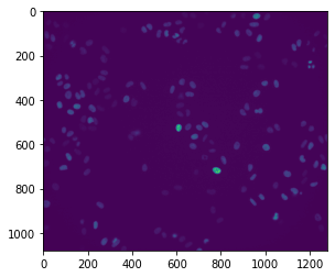
In order to viusalize the data, we will turn to matplotlib’s imshow function. This function can also be called using ax.imshow in order to plot an image as a subplot.

plt.imshow(im)

<matplotlib.image.AxesImage at 0x7fcba17b6cd0>

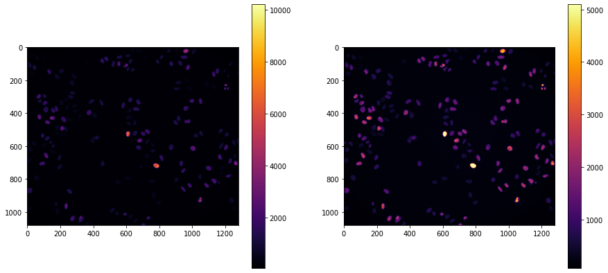
This function supports a variety of keyword arguments that include changing the colormap used to display the image and changing the minimum and maximum values that scale the colormap. Matplotlib will generally default to using the viridis colormap, but we can choose from a range of options supported by matplotlib. As an example, we will switch to using the inferno colormap and look at the effect of changing the minimum and maximum scaling values.

np.max(im),np.min(im)

(10195, 76)

# Setup two subplots to compare the impact of changing vmin and vmax
fig,ax = plt.subplots(1,2,figsize=(15,7))

# Store the output of imshow in order to set up a colorbar for that suplot
cb0 = ax[0].imshow(im, cmap='inferno')
fig.colorbar(cb0, ax=ax[0])

cb1 = ax[1].imshow(im, cmap='inferno', vmin=np.min(im), vmax=np.max(im)/2)
fig.colorbar(cb1, ax=ax[1])

<matplotlib.colorbar.Colorbar at 0x7fcba0d88a90>

Proprietary File Formats

Most microscopes store data using proprietary file formats designed by the manufacturer of the microscope, such as lif (Leica), nd2 (Nikon) and czi (Zeiss).

The Open Microscopy Environment (OME) is a consortium spanning academia and industry that produces open source software and format standards for microscopy data. They develop Bioformats which is a critical library for reading and writing the vast majority of biological image data types. You may have encountered the Bioformats plugin for Fiji which enables to Fiji to open practically any file you throw at it. Python support for Bioformats is limited, but CellProfiler has published a python wrapper for the core Java library underlying Bioformats.

Large dataset formats

Ultimately large image datasets are generally stored in one of two ways:

1. As a directory of individual fields of view (FOV) in a generally accessible format such as tiff. Information regarding the channel, z position or t step captured in each file is typically encoded in the file name such that high dimensional datasets can be reconstructed from individual files.

2. As a multidimensional hyperstack containing the entire dataset within a single file. There are many choices for this type of file format, but numpy’s file format npz is a common choice. h5 files by HDF5 are also favored for the flexibility of data organization within each file.

Image Transformations

In the course of training a machine learning model, we can augment the training dataset by performing image transformations to present the model with the same data in a new form. These transformations can take the form of reflections, rotations, scaling and others. In its simplest form, any transformation can be applied to an image by multiplying it with an appropriate transformation matrix. We will briefly review the linear algebra behind transformation matrices before looking at code examples.

For this discussion, we will consider the point $P(x,y) = \begin{bmatrix}x&y\end{bmatrix}$. Any transformation matrix is a modification of the identity matrix $$

(1)\[\begin{bmatrix} 1 & 0 \\ 0 & 1 \\ \end{bmatrix}\]

$$

For each code example, we will apply the transformation to a 1x1 square whose bottom left corner is the origin.

points = np.array([[0,0],[1,1],[0,1],[1,0]])

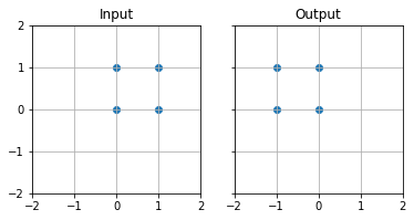
Reflection

In order to reflect $P(x,y)$ across the x axis

$$

(2)\[\begin{bmatrix}x & y\end{bmatrix}\]

(3)\[\begin{bmatrix} -1 & 0\\ 0 & 1\\ \end{bmatrix}\]

=

(4)\[\begin{bmatrix}-x & y\end{bmatrix}\]

$$

# Define transformation matrix
M = np.array([
    [-1,0],
    [0,1]
])

# Use matrix multiplication @ to multiply points by the transformation matrix
rot = points @ M

fig,ax = plt.subplots(1,2,sharey=True,sharex=True)

for i,(d,t) in enumerate(zip([points,rot],['Input','Output'])):
    ax[i].scatter(d[:,0],d[:,1])
    ax[i].set_title(t)
    
    ax[i].set_aspect('equal')
    ax[i].grid(True)
    ax[i].set_xlim(-2,2)
    ax[i].set_ylim(-2,2)

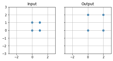
Scale

In order to scale $P(x,y)$ by a factor of 2

$$

(5)\[\begin{bmatrix}x & y\end{bmatrix}\]

(6)\[\begin{bmatrix} 2 & 0\\ 0 & 2\\ \end{bmatrix}\]

=

(7)\[\begin{bmatrix}2x & 2y\end{bmatrix}\]

$$

# Define transformation matrix
M = np.array([
    [2,0],
    [0,2]
])

# Use matrix multiplication @ to multiply points by the transformation matrix
rot = points @ M

fig,ax = plt.subplots(1,2,sharey=True,sharex=True)

for i,(d,t) in enumerate(zip([points,rot],['Input','Output'])):
    ax[i].scatter(d[:,0],d[:,1])
    ax[i].set_title(t)
    
    ax[i].set_aspect('equal')
    ax[i].grid(True)
    ax[i].set_xlim(-3,3)
    ax[i].set_ylim(-3,3)

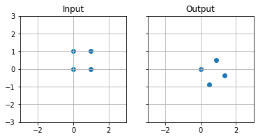
Rotation

In order to rotate $P(x,y)$ around the origin by the angle $\theta$

$$

(8)\[\begin{bmatrix}x & y\end{bmatrix}\]

(9)\[\begin{bmatrix} \cos{\theta} & -\sin{\theta}\\ \sin{\theta} & \cos{\theta}\\ \end{bmatrix}\]

$$

# Define transformation matrix
theta = np.pi/3
M = np.array([
    [np.cos(theta),-np.sin(theta)],
    [np.sin(theta),np.cos(theta)]
])

# Use matrix multiplication @ to multiply points by the transformation matrix
rot = points @ M

fig,ax = plt.subplots(1,2,sharey=True,sharex=True)

for i,(d,t) in enumerate(zip([points,rot],['Input','Output'])):
    ax[i].scatter(d[:,0],d[:,1])
    ax[i].set_title(t)
    
    ax[i].set_aspect('equal')
    ax[i].grid(True)
    ax[i].set_xlim(-3,3)
    ax[i].set_ylim(-3,3)

We will revisit transformation matrices again when we begin peparing augmented data for model training.

---

%load_ext watermark
%watermark -u -d -vm --iversions

Last updated: 2021-04-28

Python implementation: CPython
Python version       : 3.7.10
IPython version      : 5.5.0

Compiler    : GCC 7.5.0
OS          : Linux
Release     : 4.19.112+
Machine     : x86_64
Processor   : x86_64
CPU cores   : 2
Architecture: 64bit

numpy     : 1.19.5
IPython   : 5.5.0
matplotlib: 3.2.2