Optimizers

Optimizers#

In this notebook, we will go over the different optimizers used to train deep learning models. These include, SGD with momentum, Adagrad, RMS Prop, and Adam.

This notebook should (hopefully) give you some understanding about differences between the different optimizers. If you’re in doubt about what optimizer to use, Adam is good first start.

Load packages#

Import the packages needed for this notebook.

import numpy as np
from tqdm import tqdm
from skimage.measure import find_contours
from plotly.subplots import make_subplots
import plotly.graph_objects as go
import plotly.io as pio
from plotly import colors

pio.renderers.default = "notebook"

Create toy loss landscape#

To visualize how the different models train, we will implement a toy loss landscape. The landscape that will use is the loss for a linear classifier for sklearn’s moons dataset. For this dataset, we will have a collection of 2-D points ($X_0$ and $X_1$) and the associated labels. The probability of being in each class is given by:

\[\begin{align*} p_0 &= \frac{e^{-(w_0 x_0 + w_1 x_1)}}{1+e^{-(w_0 x_0 + w_1 x_1)}}, \\ p_1 &= \frac{1}{1+e^{-(w_0 x_0 + w_1 x_1)}} \end{align*}\]

The linear classifier can be viewed as the equivalent of a Dense layer (with two outputs) followed by a softmax layer. It is also the equivalent of logistic regression. For training, we will randomly initialize the weights - e.g., we will start at a random point on this landscape and then see how each optimizer traverses it.

from sklearn.datasets import make_moons
X, y = make_moons(1000, noise=0.1)

def logistic(x, w):
    alpha = 1 + np.exp(-x[:,0]*w[0] - x[:,1]*w[1])
    p_0 = (alpha-1)/alpha
    p_1 = 1/alpha
    
    p = np.stack([p_0, p_1], axis=-1)
    grad_dict = {}
    grad_dict['p0_w0'] = -x[:,0]*(alpha-1) / alpha**2
    grad_dict['p0_w1'] = -x[:,1]*(alpha-1) / alpha**2
    grad_dict['p1_w0'] = - grad_dict['p0_w0']
    grad_dict['p1_w1'] = - grad_dict['p0_w1']
    
    return p, grad_dict

def loss(x, y, w):
    p, grad_dict = logistic(x, w)
    
    # Compute losses - get p_correct
    p_correct = p[np.arange(y.shape[0]),y]
    losses = -np.log(p_correct)
    losses = np.mean(losses, axis=0)
    
    # Compute gradient
    grad_w0 = np.stack([grad_dict['p0_w0'], grad_dict['p1_w0']], axis=-1)
    grad_w1 = np.stack([grad_dict['p0_w1'], grad_dict['p1_w1']], axis=-1)
    
    grad_w0 = grad_w0[np.arange(y.shape[0]),y]
    grad_w1 = grad_w1[np.arange(y.shape[0]),y]
    
    grad_w0 = -1/p_correct*grad_w0
    grad_w1 = -1/p_correct*grad_w1
    
    grad_w0 = np.mean(grad_w0, axis=0)
    grad_w1 = np.mean(grad_w1, axis=0)
    
    grad = np.stack([grad_w0, grad_w1], axis=-1)
    
    return losses, grad

# Compute loss landscape
w0_range = np.arange(-10, 10, 0.1)
w1_range = np.arange(-10, 0, 0.05)

losses_array = np.zeros((w0_range.shape[0], w1_range.shape[0]))
for i, w0 in tqdm(enumerate(w0_range)):
    for j, w1 in enumerate(w1_range):
        l, _ = loss(X, y, [w0,w1])
        losses_array[i,j] = l

200it [00:06, 30.99it/s]

We can take a quick look at the dataset we are working with and the loss landscape.

# Visualize the data and loss landscape
fig = make_subplots(rows=1, cols=2, subplot_titles=('Data Points','Loss Landscape'))

color_list = ['blue' if i else 'red' for i in y]
fig.add_trace(
    go.Scatter(
        x=X[:,0],
        y=X[:,1],
        mode='markers',
        marker_color=color_list
    ),
    row=1,col=1
)
fig.update_xaxes(title_text='$X_0$',row=1,col=1)
fig.update_yaxes(title_text='$X_1$',row=1,col=1)

fig.add_trace(
    go.Contour(
        x=w0_range,
        y=w1_range,
        z=losses_array.T,
        contours_coloring='lines',
        line_width=2,
        showscale=False,
        colorscale='Viridis',
        contours=dict(
            start=0.3,
            end=6.2,
            size=0.5,
            showlabels=True,
        )
    ),
    row=1,col=2
)
fig.update_xaxes(title_text='$W_0$',row=1,col=2)
fig.update_yaxes(title_text='$W_1$',row=1,col=2)

fig.update_layout(showlegend=False)
fig.show()

Prepare utilities for visualization#

In order to simplify visualizations, we will calculate the contours of the loss landscape and prep a utility function for calculating colors for the contours. You can toggle these code cells if you are interested in seeing the code in detail.

Show code cell content Hide code cell content

optimizers = {}

def initialize_w():
    w_0 = np.random.uniform(low=-10, high=10)
    w_1 = np.random.uniform(low=-10, high=0)
    w = np.stack([w_0, w_1], axis=-1)
    return w

def visualize(losses, ws):
    fig = make_subplots(rows=1, cols=2, subplot_titles=('Loss History','Loss Landscape'))
    
    # Downsample data by every 100th point
    ls = losses[::100]
    ws = ws[::100]
    times = np.arange(len(losses))[::100]
    
    ## Subplot 1
    # Trace 0 loss history
    fig.add_trace(
        go.Scatter(
            x=times,
            y=ls,
            mode='lines',
            line=dict(color=linecolor)
        )
    )

    # trace 1 time bar
    fig.add_trace(
        go.Scatter(
            x=[10,10],
            y=[0,10],
            mode='lines',
            line=dict(color=timecolor)
        )
    )
    
    ## Subplot 2
    # trace 2 loss trajectory
    fig.add_trace(
        go.Scatter(
            x=ws[:,0],
            y=ws[:,1],
            line=dict(color=linecolor)
        ),
        row=1,col=2
    )

    # trace 3 loss time tracker
    fig.add_trace(
        go.Scatter(
            x=np.array([ws[0,0]]),
            y=np.array([ws[0,1]]),
            marker_size=10,
            line=dict(color=timecolor)
        ),
        row=1,col=2
    )
    
    # Plot loss landscape contours
    for i,l in enumerate(normlevels):
        fig.add_trace(
            go.Scatter(
                x=contour_X[i],
                y=contour_Y[i],
                text='Level {}'.format(levels[i]),
                line=dict(color=get_continuous_color(colorscale,l))
            ),
            row=1,col=2
        )
    
    # Define animation frames
    nframes = times.shape[0]
    frames = [dict(
        name = t,
        data = [
            go.Scatter(x=np.array([times[t],times[t]]),y=np.array([0,10])),
            go.Scatter(x=np.array([ws[t,0]]),y=np.array([ws[t,1]]))
        ],
        traces = [1,3]
    ) for t in range(nframes)]
    
    # Define play button
    updatemenus = [dict(
        type='buttons',
        buttons=[dict(
            label='Play',
            method='animate',
            args=[
                None,
                dict(mode='immediate',
                     fromcurrent=True,
                     frame=dict(duration=50))
            ]
        )]
    )]
    
    # Update figure with new info
    fig.update(frames=frames)
    fig.update_layout(updatemenus=updatemenus)
    fig.update_layout(showlegend=False)
    fig.update_xaxes(title_text='$W_0$',range=[-10,10],row=1,col=2,autorange=False)
    fig.update_yaxes(title_text='$W_1$',range=[-10,0],row=1,col=2,autorange=False)
    fig.update_xaxes(title_text='Iteration',row=1,col=1)
    fig.update_yaxes(title_text='Loss',row=1,col=1)
    
    fig.show()

w_init = initialize_w()

SGD#

Lets briefly recall how stochastic gradient descent works. Our model, which has parameters $W$ takes training data $X$ as inputs and produces predictions $\hat{y}$. Our loss function compares these predictions with the ground truth values $y$ and produces a score that tells us how well we did - a low value of the loss means we did well, while a high value means we did poorly. While the loss function can be written as $L(y, \hat{y})$, the fact that our model produces $\hat{y}$ means that there is an implicit functional dependence on the model parameters $W$ - e.g. the loss function can be written as $L(X, y, W)$.

Assuming our model and our loss are differentiable functions, we can use gradient descent to solve our problem. To do this we must do the following

Randomly pick initial parameters $W$
Compute the gradient $\nabla W$ for our training data
Update the weights $W \rightarrow W - lr * \nabla W$, where lr is the learning rate
Repeat until convergence

There is one point we glossed over in our earlier discussion that is relevent here - selecting the training data for computing our gradients. There are essentially three options we can choose from

Compute the gradient on the whole training dataset for each step. Concretely, this means we compute the gradient for each example and use the mean gradient to update the weights. This allows each item of the dataset to contribute, but has the drawback of having high memory requirements and slow training. For most datasets and deep learning models, this isn’t feasible. Technically, this is what “gradient descent” refers to.
Compute the gradient one randomly chosen example at a time, and use the gradient from that one example to update the weights. This requires less memory, and the computation from each step is faster. However, because only one example contributed to the gradient calculation, there can be substantial noise in the gradient - this randomness in direction can slow down training. Technically, this is what “stochastic gradient descent” refers to.
Compute the gradient for a collection of examples (e.g., a batch) that are randomly chosen, and use the average gradient derived from this batch to update the weights. This achieves a balance between the first two methods - using a batch of examples reduces the stochasticity in the gradients, while keeping the memory and compute times reasonable. Technically, this is what “mini batch gradient descent” refers to.

Practically speaking, the third option is what we usually do - although for memory intensive datasets, the batch size can be set to 1, which effectively reduces it to the second option. Although it isn’t accurate, we will refer to both the second and third choices as “stochastic gradient descent,” recognizing we can set the batch size to 1.

# Implementation of SGD
def SGD(loss_function, w_init, X, y, lr = 1e-2, n_steps=int(3e4), batch_size=1):
    losses = []
    grads = []
    ws = []

    ws.append(w_init)
    
    for step in tqdm(range(n_steps)):
        # Select a random image
        i = np.random.randint(0, X.shape[0]-1, size=batch_size)
        X_batch = X[(i)]
        y_batch = y[(i)]
        
        l, g = loss_function(X_batch, y_batch, ws[-1])
        losses.append(l)
        grads.append(g)
        
        new_w = ws[-1] - lr * g
        ws.append(new_w)
        
    losses = np.stack(losses, axis=0)
    grads = np.stack(grads, axis=0)
    ws = np.stack(ws, axis=0)
    return losses, grads, ws      

# Toy optimization with visualization
losses, grads, ws = SGD(loss, w_init, X, y)
optimizers['SGD'] = [losses, ws]

100%|██████████| 30000/30000 [00:04<00:00, 6824.48it/s]

visualize(*optimizers['SGD'])

SGD with momentum#

Even with using batches of examples to compute our gradients, the noise associated with random batches can make training difficult. This noise can be particulary problematic when the the loss function is much steeper in one direction versus another. In these situations, SGD experiences oscillations, which can significantly slow down training. One can think of these oscillations as artifacts of the optimization algorithm “forgetting” the good directions it observed in the past. 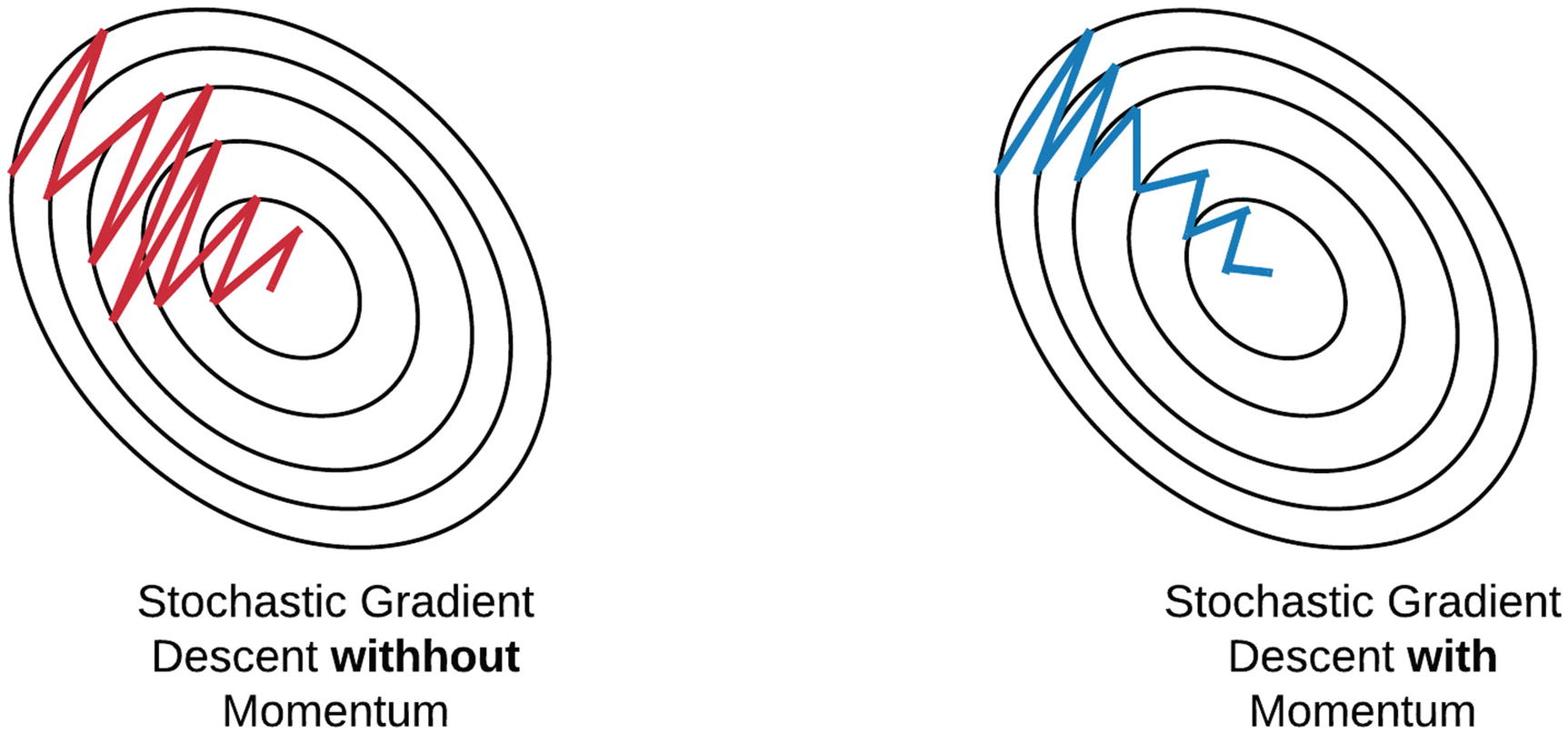Comparison of SGD with and without momentum

“Momentum” seeks to rectify this by using an average of recent gradients to update the weights, rather than using the gradients from just one batch. The term momentum comes from an anology of a ball rolling down a hill. If a ball rolls in the same direction (e.g., down), then it gains momentum. Similarly, if there is a consistent direction that improves training, the momentum update rule will keep the weights moving in that direction. By using an exponential average of the gradients, there is now a mechanism for “remembering” good directions - if a direction is good it is likely to appear repeatedly during training and will be captured by the exponential average.

Mathematically, the update formula is given by:

\[\begin{align*} m_t &= m_{t-1} * \beta + \nabla W * (1-\beta) \\ W_t &= W_{t-1} - lr * m_t \end{align*}\]

# Implementation of SGD with momentum
def SGDMomentum(loss_function, w_init, X, y, lr=1e-2, beta=0.9, n_steps=int(3e4), batch_size=1):
    losses = []
    grads = []
    m = None
    ws = []
    
    ws.append(w_init)
    
    for step in tqdm(range(n_steps)):
        # Select a random image
        i = np.random.randint(0, X.shape[0]-1, size=batch_size)
        X_batch = X[(i)]
        y_batch = y[(i)]
        
        l, g = loss_function(X_batch, y_batch, ws[-1])
        losses.append(l)
        grads.append(g)
        
        if m is None:
            m = g
        else:
            m = beta * m + (1-beta) * g
            
        new_w = ws[-1] - lr* m
        ws.append(new_w)
        
    losses = np.stack(losses, axis=0)
    grads = np.stack(grads, axis=0)
    ws = np.stack(ws, axis=0)
        
    return losses, grads, ws

# Toy optimization with visualization
losses, grads, ws = SGDMomentum(loss, w_init, X, y)
optimizers['SGDMomentum'] = [losses, ws]

100%|██████████| 30000/30000 [00:04<00:00, 6894.18it/s]

visualize(*optimizers['SGDMomentum'])

Adagrad#

Adagrad is short for adaptive gradients. It seeks to solve the same problem as momentum, but in a different way. Adagrad effectively defines a separate learning rate for each parameter by normalizing the learning rate by a running sum of the square of the gradients. The effect of this scheme is as follows: if a parameter is experiencing large gradients, then the learning rate is reduced because the running sum will be large. If a parameter is experiencing small gradients, then the learning rate will be higher because the running sum will be low. By normalizing the gradients in this way, we can combat the negative effects of having learning rates that are too high or too low. Moreover, we can do this in a way thats customized to each parameter.

Mathematically, the update formula is given by:

\[\begin{align*} cache_t &= cache_{t-1} + \left( \frac{\partial Loss}{\partial W_{t-1}} \right)^2, \\ W_t &= W_{t-1} - \frac{lr}{\sqrt{cache_t} + \epsilon}\frac{\partial Loss}{\partial W_{t-1}} \end{align*}\]

# Implementation of Adagrad
def Adagrad(loss_function, w_init, X, y, lr=1e-2, n_steps=int(1e6), epsilon=1e-5, batch_size=1):
    losses = []
    grads = []
    cache = None
    ws = []
    
    ws.append(w_init)
    
    for step in tqdm(range(n_steps)):
        # Select a random image
        i = np.random.randint(0, X.shape[0]-1, size=batch_size)
        X_batch = X[(i)]
        y_batch = y[(i)]
        
        l, g = loss_function(X_batch, y_batch, ws[-1])
        losses.append(l)
        grads.append(g)
        
        if cache is None:
            cache = g**2
        else:
            cache += g**2
        
        new_w = ws[-1] - lr / (np.sqrt(cache) + epsilon) * g
        ws.append(new_w)
        
    losses = np.stack(losses, axis=0)
    grads = np.stack(grads, axis=0)
    ws = np.stack(ws, axis=0)
        
    return losses, grads, ws

# Toy optimization with visualization
losses, grads, ws = Adagrad(loss, w_init, X, y)
optimizers['Adagrad'] = [losses, ws]

100%|██████████| 1000000/1000000 [02:38<00:00, 6315.70it/s]

visualize(*optimizers['Adagrad'])

RMS Prop#

RMSProp is almost identical to Adagrad, but the difference lies in how the cache is implemented. Rather than keep a running sum, RMS prop computes an exponential average of the squared gradient and uses this exponential average to normalize the learning rate. This means the learning rate is normalized based on what happened recently in training, rather than the sum total of the training trajectory. This mitigates one of adagrads weaknesses, which is slow training due to perpetually increasing cache values.

Mathematically, the update formula is given by:

\[\begin{align*} cache_t &= \rho * cache_{t-1} + (1-\rho)\left( \frac{\partial Loss}{\partial W_{t-1}} \right)^2, \\ W_t &= W_{t-1} - \frac{lr}{\sqrt{cache_t} + \epsilon}\frac{\partial Loss}{\partial W_{t-1}} \end{align*}\]

# Implementation of RMSProp
def RMSProp(loss_function, w_init, X, y, lr=1e-2, rho=0.9, n_steps=int(3e4), epsilon=1e-5, batch_size=4):
    losses = []
    grads = []
    cache = None
    ws = []
    
    ws.append(w_init)
    
    for step in tqdm(range(n_steps)):
        # Select a random image
        i = np.random.randint(0, X.shape[0]-1, size=batch_size)
        X_batch = X[(i)]
        y_batch = y[(i)]
        
        l, g = loss_function(X_batch, y_batch, ws[-1])
        losses.append(l)
        grads.append(g)
        
        if cache is None:
            cache = g**2
        else:
            cache = rho*cache + (1-rho)*g**2
        
        new_w = ws[-1] - lr / (np.sqrt(cache) + epsilon) * g
        ws.append(new_w)
        
    losses = np.stack(losses, axis=0)
    grads = np.stack(grads, axis=0)
    ws = np.stack(ws, axis=0)
        
    return losses, grads, ws

# Toy optimization with visualization
losses, grads, ws = RMSProp(loss, w_init, X, y)
optimizers['RMSProp'] = [losses, ws]

100%|██████████| 30000/30000 [00:03<00:00, 7515.19it/s]

visualize(*optimizers['RMSProp'])

Adam#

Adam is short for adaptive moment estimation, and can be thought of as a fusion of momentum and RMSProp. Momentum uses a running exponential average of the gradients to update the weights (e.g., to keep moving in good directions). RMSProp scales the learning rate for each parameter. Adam does both steps in its update rule to get the benefits of both methods.

Mathematically, the update formula is given by:

\[\begin{align*} m_t &= \beta_1 * m_{t-1} + (1-\beta_1)\frac{\partial Loss}{\partial W_t},\\ cache_t &= \beta_2 * cache_{t-1} + (1-\beta_2)\left( \frac{\partial Loss}{\partial W_{t-1}} \right), \\ \hat{m}_t &= \frac{m_t}{1-\beta_1^t}, \\ \hat{cache}_t &= \frac{cache_t}{1-\beta_2^t}, \\ W_t &= W_{t-1} - \frac{lr}{\sqrt{\hat{cache}_t} + \epsilon}\hat{m}_t \end{align*}\]

The terms in the hat are introduced to correct for initializing the moments and cache with zero values. We don’t do that initialization for the other implementations, but we do it here for those who wish to follow along the original Adam paper.

# Implementation of Adam
def Adam(loss_function, w_init, X, y, lr=1e-2, beta_1=0.9, beta_2=0.99, n_steps=int(3e4), epsilon=1e-5, batch_size=1):
    losses = []
    grads = []
    m = 0
    cache = 0
    ws = []
    
    ws.append(w_init)
    
    for step in tqdm(range(n_steps)):
        # Select a random image
        i = np.random.randint(0, X.shape[0]-1, size=batch_size)
        X_batch = X[(i)]
        y_batch = y[(i)]
        
        l, g = loss_function(X_batch, y_batch, ws[-1])
        losses.append(l)
        grads.append(g)
        
        if m is None:
            m = g
        else: m = beta_1 * m + (1-beta_1)*g
            
        if cache is None:
            cache = g**2
        else:
            cache = beta_2*cache + (1-beta_2)*g**2
            
        m_hat = m / (1-beta_1**(step+1))
        cache_hat = cache / (1-beta_2**(step+1))
        
        new_w = ws[-1] - lr / (np.sqrt(cache) + epsilon) * m
        ws.append(new_w)
        
    losses = np.stack(losses, axis=0)
    grads = np.stack(grads, axis=0)
    ws = np.stack(ws, axis=0)
        
    return losses, grads, ws

# Toy optimization with visualization
losses, grads, ws = Adam(loss, w_init, X, y)
optimizers['Adam'] = [losses, ws]

100%|██████████| 30000/30000 [00:04<00:00, 6064.90it/s]

visualize(*optimizers['Adam'])

Comparison of all optimizers#

Finally we can look at a comparison of each optimizer side by side.

Show code cell source Hide code cell source

# Gallery of plots with one per optimizer
fig = make_subplots(rows=2, cols=5,shared_yaxes=True,subplot_titles=list(optimizers.keys()))

# Downsample data by every 100th point
times = np.arange(len(losses))[::100]

for j,opt in enumerate(optimizers.keys()):
    j = j+1
    ls = optimizers[opt][0][::100]
    ws = optimizers[opt][1][::100]
    
    # Plot loss landscape contours
    for i,l in enumerate(normlevels):
        fig.add_trace(
            go.Scatter(
                x=contour_X[i],
                y=contour_Y[i],
                text='Level {}'.format(levels[i]),
                line=dict(color=get_continuous_color(colorscale,l)),
                showlegend=False,
                opacity=0.6
            ),
            row=1,col=j
        )
    
    # Loss trace
    fig.add_trace(
        go.Scatter(
            x=ws[:,0],
            y=ws[:,1],
            name=opt,
            legendgroup=opt,
            line=dict(color=linecolor)
        ),
        row=1,col=j
    )
    
    # Loss history
    fig.add_trace(
        go.Scatter(
            x=times,
            y=ls,
            mode='lines',
            name=opt,
            legendgroup=opt,
            showlegend=False,
            line=dict(color=linecolor)
        ),
        row=2,col=j
    )
    
    fig.update_xaxes(range=[-10,10],row=1,col=j,autorange=False)
    fig.update_yaxes(range=[-10,0],row=1,col=j,autorange=False)
    fig.update_xaxes(title_text='Iteration',row=2,col=j)
    
# Get current trace index
tindex = len(fig.data)
traces = []

# Add time traces
for j,opt in enumerate(optimizers.keys()):
    j = j+1
    # All lines start in the same place
    fig.add_trace(
        go.Scatter(
            x=[10,10],
            y=[0,10],
            mode='lines',
            line=dict(color=timecolor)
        ),
        row=2,col=j
    )
    traces.append(tindex)
    tindex += 1

    # trace 3 loss time tracker
    fig.add_trace(
        go.Scatter(
            x=np.array([ws[0,0]]),
            y=np.array([ws[0,1]]),
            marker_size=10,
            showlegend=False,
            line=dict(color=timecolor)
        ),
        row=1,col=j
    )
    traces.append(tindex)
    tindex += 1

# Define animation frames
nframes = times.shape[0]
frames = []
for t in range(nframes):
    f = dict(
        name = t,
        traces = traces,
        data = []
    )
    for j,opt in enumerate(optimizers.keys()):
        j = j+1
        ws = optimizers[opt][1][::100]
        # Append time bar
        f['data'].append(go.Scatter(x=np.array([times[t],times[t]]),y=np.array([0,10])))
        # Append time dot
        f['data'].append(go.Scatter(x=np.array([ws[t,0]]),y=np.array([ws[t,1]])))

    # Add completed frame to list
    frames.append(f)

# Define play button
updatemenus = [dict(
    type='buttons',
    buttons=[dict(
        label='Play',
        method='animate',
        args=[
            None,
            dict(mode='immediate',
                 fromcurrent=True,
                 frame=dict(duration=20))
        ]
    )]
)]

# Update figure with new info
fig.update(frames=frames)
fig.update_layout(updatemenus=updatemenus)
fig.update_layout(showlegend=False)
fig.update_yaxes(title_text='Loss',range=[0,10],autorange=False,row=2,col=1)
fig.show()

%load_ext watermark
%watermark -u -d -vm --iversions

Last updated: 2021-04-28

Python implementation: CPython
Python version       : 3.7.10
IPython version      : 5.5.0

Compiler    : GCC 7.5.0
OS          : Linux
Release     : 4.19.112+
Machine     : x86_64
Processor   : x86_64
CPU cores   : 2
Architecture: 64bit

numpy  : 1.19.5
plotly : 4.4.1
IPython: 5.5.0

Optimizers

Contents

Optimizers#

Load packages#

Create toy loss landscape#

Prepare utilities for visualization#

SGD#

SGD with momentum#

Adagrad#

RMS Prop#

Adam#

Comparison of all optimizers#